4 Algebraic position determination

links → HOME, chapter 1, chapter 2, chapter 3, chapter 5 and 6, chapter 7, chapter 8

The most important German navigation teacher Friedrich August Arthur Breusing (1818-1892) was not a friend of graphic navigation methods and therefore rejected the Sumner method. Even in his textbook „Steuermannskunst“ (The Art of Navigation), which appeared in many editions well into the 20th century even after his death as the standard work of German ocean navigation, he only included Saint Hilaire’s graphic method in a later edition. But only because this method was already very widespread.
That the Gauss method was not even mentioned in any of the ten editions of his textbook is at least remarkable. It can hardly be assumed that Breusing, as director of the leading German navigation school at the time, which was the helmsman’s school in Bremen, did not know about the Gauss method. Yet this very method is the most brilliant analytical piece of the solution of the two-height problem ever.
Rigorous analytical methods, although mathematically exact in contrast to the graphical approximation methods, could not be used in his day because there were no computers. In spite of the proliferation of the new graphical methods, which had the ambition to supersede everything old, he still included Borda’s and Lalande’s method in the 5th edition of his textbook. Borda’s method is not a strictly analytical method, but an iterative method, but it is at least not graphical.
In the following we will deal with the mathematically exact methods. In doing so, we cannot avoid the use of spherical trigonometry. But this is simpler than some might think. Therefore, we will first turn to some things of spherical geometry.

4.1 A Bit of Mathematics

Now please don’t get a fright – I know that mathematics is a non-word for many. But if mathematics is presented well, it can even inspire many people and will hardly put anyone off. In the following, we also want to present it in a way that everyone can understand. The French mathematician and philosopher Jean-Baptist le Rond d’Alembert had the following opinion about mathematics:

„Mathematics is a kind of toy which nature has thrown at us for consolation and entertainment in the darkness.“

In fact, a single formula is sufficient for a comprehensive understanding of all methods of astronavigation, whether they are those of Borda, Sumner, Hilaire or others, and it is not even complicated. It is only always presented in a complicated way, as if some authors wanted to show what they can do. We would like to avoid this here as far as possible. The formula is called the cosine side theorem and is used to calculate either a side or an angle in a triangle on the surface of a sphere.
Let us first look at Figure 4.1 on the left. It shows a sphere whose surface is covered by three great circles of the same diameter as the sphere. The three circular lines edge a total of eight possible triangles of different sizes on the surface of the sphere, but we will only take a closer look at one of the two smaller ones.
As in the geometry of the plane, the corners are marked with the capital letters ABC, the sides with the lower case letters abc and the angles between the sides with the Greek letters α β γ. We will notice an essential difference to a triangle in the plane in a moment. While side lengths of a triangle in the plane are measured in centimetres, metres or miles, the side lengths of a spherical triangle are measured in degrees.

You can see how this happens in Figure 4.1 on the right. An angle b at the centre of the sphere spans an arc of a circle with a length of b on the surface of the sphere. However, the length of the arc is not primarily measured in metres, inches or any other length measure, but in the same degree measure as the angle b in the centre of the earth. The length of the arc b is the so-called radian measure of the angle b in the centre of the sphere. Both are measured in degrees and have the same number of degrees.

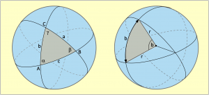
Thus everything is relative in spherical trigonometry. Whether the side of a spherical triangle is viewed on a marble or on the earth’s sphere is irrelevant for the time being. If a calculated arc has a length of 3 degrees, then this is 180 nautical miles to be covered on the globe and not even a millimetre on the marble. But this is exactly what makes spherical trigonometry sometimes so simple and also so interesting.
We notice that only circles are involved here. Angles at the centres of circles are, however, also necessary to be able to define arcs of circles, as shown in Figure 4.1 on the right with the angle b and the arc of a circle b. For this reason, all sides and angles used in calculations are circular functions. Circular functions are the sine and cosine functions.
Why this has to be the case will not be discussed further at this point. It follows that if we want to calculate the side b from the sides a, c and the angle β of a spherical triangle, we can only do this with the circular functions of these three elements. So we do not calculate with the side a, but with cos(a) or sin(a). For the side c, cos(c) or sin(c) then applies and instead of the angle β we use cos(β) or sin(β). Whether the cosine or the sine is to be used is shown by the rules of the cosine side theorem below. We will leave aside the way in which this formula was once derived. Of course, we do not get a side or an angle as a result, but only the cosine or sine of a side or an angle in a circular function.
But how do we get from cos(b) back to b or from sin(β) to β at the end? It’s quite simple with the inverse function, which is called the arc function (Latin arcus = arc) and is extremely easy to handle.
If we want to calculate a side, for example the side b, but only have a formula to calculate cos(b), then this is no problem. We replace the cosine with the arc cosine. Here is an example: If we have

   

but want to work out b, then we simply rewrite the formula and get

   

We will omit the brackets around the arguments in future. So we will write sin instead of sin() and instead of arccos we can also write cos^-1. This notation is mainly used on pocket calculators. If we have the number 0.9993908 for cos b in the display, then we can simply press the cos^-1 key on many models. The display then shows the number 2, which is then 2°.

4.1.1 The Cosine Side Set

The cosine side theorem is used in two variants. The first variant is used when one side of a triangle is to be calculated. For this, the other two sides and the angle between these sides must be known. In order to be able to calculate the side b in Figure 4.2, one therefore needs the sides s and p as well as the angle ψ (psi) enclosed by them. The calculation formula for this is:

   

or as rule 1 in words:

The cosine of one side is equal to the product of the cosines of the other two sides added by the product of the sines of these two sides multiplied by the cosine of the intermediate angle.

If one wants to calculate an angle, then all sides must be known. To calculate the angle in Figure 4.2, the following formula must be applied:

   

or as Rule 2 in words:

The cosine of an angle is equal to the cosine of the side opposite the angle, minus the product of the cosines of the remaining sides, and this all divided by the product of the sines of the remaining sides.

In principle, this is already the whole scope of spherical trigonometry as it is used in astronavigation. Now we only have to define the sizes b, p and s, because we don’t know them yet. We only know the latitude as estimated latitude or DR latitude, furthermore the declination δ and the horizon distance h measured with a sextant.
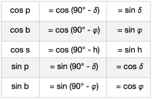
At this point, the complement relations come into play as simplifications. A complement angle or simply the complement of an angle is its supplement to 90°. If an angle has a magnitude of 60°, then its complement angle is 30°. Because the distance from the equator to the pole is always 90°, in Figure 4.2 the declination δ is the complement of side p and the complement of side b on the observation meridian is the latitude . The following table shows all the complements that apply here.

With the complements of the sides we get access to the true sides in the first place. We don’t know how long the sides b, s or p are in order to calculate . But with the complements, the supplements to 90°, this is quite easy. Instead of the unknown side cos p, the known declination sin δ is inserted, which is absolutely the same.

This simplifies the formulae. Without this, the expression cos (90° – δ) would have to be inserted in the equations for cos p and the expression sin (90° – δ) for sin p. The result would be long formula expressions. The result would be long formula expressions. The table shows the sides in the first column and the complements of the sides in the third column.

Using the complements, we then exchange everything and get the new formula for calculating side b:

   

We could now use the arc cosine function to calculate the radian of side b, subtract this from 90° and we would have the latitude . But it is even simpler. The complements in the table show that cos b is equal to sin . Therefore, we use arcsin instead of arccos and get the latitude directly, as the following formula shows:

(4.1)  

Instead of arcsin, sin^-1 can also be written.
In the second formula for calculating the polar angle we exchange the elements s, p and b for the complements h, δ and and get:

   

We get the polar angle itself here with the arc cosine function:

(4.2)  

But how do the complement relations explain themselves? This is due to the course of the circular functions sine and cosine, which can be seen in figure 4.3 over one oscillation period. The course of the curves continues infinitely into the positive and negative. The amplitude only varies between +1 and -1. The phase difference in the courses of both curves, which is exactly 90°, is clearly recognizable. The function value 1 or 0 of both curves differs by 90°. If the cosine curve has the value 1, then the sine curve has it 90° after or before. This does not only apply to 0 and 1, but all function values of the two circular functions permanently differ by 90°.

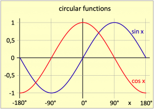
Other important properties are that the cosine curve is symmetrical to the zero axis. It follows that the function values of positive and negative angles with the same name are identical. It applies cos(+x) = cos(-x). For the sine curve, the function values of positive and negative angles with the same name have an opposite sign, i.e. sin(+x) = – sin(-x).

Now this is really all the mathematics that is sufficient to describe and understand all the known classical methods of astronomical navigation and, if you want to, to calculate them.
If someone has to use a sextant to find their way home, which has happened before, even a mobile phone won’t help for long because the battery will run out after a few days if there is no solar charger on board. There have also been cases where a boat was stuck in the tidal flats for days and the sea rescuers could not be informed of its position because both the skipper and the crew had forgotten their mobile phones. A sextant, equation 4.2, a nautical yearbook and a wristwatch could already help here – and of course a calculator.
The latitude is obtained from the noon latitude. From this and from the altitude of the sun measured a few hours later and the declination from the Nautical Almanac, the hour angle is calculated using equation 4.2, which is quickly typed together on a calculator. The Nautical Almanac, which you should have on board, also gives the GHA and if the hour angle is subtracted from this (it is afternoon), you have the longitude of the position and could give the position to the sea rescuers.
This was not intended to be a guide for a simple back-up, but merely to show how simple astronavigation actually is. Incidentally, this is exactly the procedure James Cook used to navigate throughout his second voyage. He did not have a Nautical Almanac, but he did have declination tables and equation of time tables. He got the GHA by adding the equation of time to the difference between chronometer time and 12:00 GMT and multiplying the result by the sun’s angular velocity of 15°/h – quite elaborate.
His journey began in 1772 and lasted three years. In the process, he covered more than 300 000 km. His mission was to search for Antarctica, which he did not find and instead produced the first and amazingly precise map of the South Sea Islands. The chronometer he used was an exact replica of the H4 shown in Figure 1.5. He was not allowed to take the original H4 by John Harrison with him because, as a result of being dismantled several times before the Longitude Commission, it was no longer suitable for this voyage. The London watchmaker Larcum Kendall made an exact copy for this purpose according to Harrison’s instructions, which was later given the designation K1. James Cook referred to Harrison’s invention as „our never-failing guide“ or „our reliable friend“.
Because the latitude was always only estimated in this procedure, it can deviate from the true latitude. If one repeats the same calculation with only one more latitude, then one obtains a different longitude on this second estimated latitude and thus a second possible position. If you draw a line through both possible locations, then this is a position line, because somewhere but on this line will be the position of the ship. This is the very position line that Captain Sumner discovered on his memorable voyage in 1837, thus founding the era of modern astronavigation. With the invention of an accurate clock and a single simple mathematical formula, a new age dawned in the history of navigation.

Today, we no longer have to rely on manually calculating formulas to find our position, unless we want to. Computers, smartphones and tablets do the calculating. Formulas are only important for understanding matter and for software developers to write the appropriate programs for these devices. So the point of all the formulae in the articles shown here is only to describe the relationships accurately and is not intended to be a guide to practical navigation. In addition, much care has been taken to leave out academic ballast.

 

4.2 Cenith Point and Circles of Position

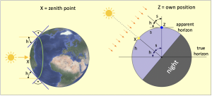
We now want to deal with two terms that are needed for further understanding. First of all, the zenith point of a celestial body, including the sun, and the question of what information the different heights or vertical distances from the horizon line give us.
On flat land or at sea, we see spires or mountains higher and higher the closer we get to them. From the angle of elevation and the known height of a building or a mountain peak, it would then be quite easy to calculate the distance.
However, the sun and stars are infinitely far away and their actual distance would not help us either. It helps us to know that the earth is a sphere. This allows us to determine the distance to the terrestrial zenith point of a star despite its huge distance. The zenith point is, so to speak, the base point of the star on the Earth’s surface. In a geometric view, one would have to connect the centres of the sun and the earth with an imaginary line. The zenith point of the sun is then the place where this imaginary line breaks through the earth’s surface. Figure 4.4 shows this schematically on the left. The position of this location is not fixed, because the Earth is rotating and thus the zenith point is racing towards the west at jet speed.
The position of the zenith point of the sun is described with an hour angle, the GHA and the declination. These position data are also called ephemerides. The Greenwich hour angle GHA counts from 0 to 360° once around the Earth, going west from the prime meridian.
The declination is the latitude of the zenith point. It changes from about 23.44° S to 23.44° N between the solstices. The cause of the declination is the oblique position of the Earth’s axis, which causes the seasons to change. How this works can be seen quite clearly in Figure 7.3.
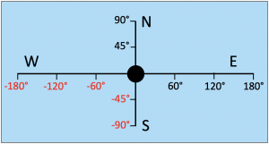
In contrast to a Cartesian coordinate system, the spherical coordinates of the Earth’s degree system are limited between 90° north and 90° south or 180° east and 180° west. West longitudes and south latitudes have negative signs.

The scale of hour angles, such as the GHA or the LHA, deviates from this, however, because they count earth-rotating from 0° to 360°. If hour angles greater than 360° or less than zero occur in a calculation, then these are carryovers and 360° must simply be subtracted or 360° added, bringing the angle back into the permissible number range.
This rule also applies to geographical longitudes, whereby the carryovers already occur when 180° is exceeded in each case. Thus, 360° have to be subtracted from an overflow to 182° E and this then becomes -178° or 178° W.
As Figure 4.4 on the left shows, all observers who are currently on the green circle line would see the sun at the same time at the same altitude h. This circle line is therefore called the altitude line. This circular line is therefore called the line of the thame altitude or better line of position, because an observer’s location is somewhere on this line. It is a circle with a spherical radius, the length of which is to be designated s.

If an observer of a celestial body stands on the circle of position the celestial body he is observing, then he is also standing on the circle of position any other celestial body that he can observe from the same place. This, after all, is the essence of astronomical navigation. The circles of Position of the two stars cross directly under the feet of the observer, and thus literally in his location. So the task is simply formulated:

To determine a position means to determine the points of intersection of two observed circles of Position.

The same works with altitude circles of only one celestial body, such as the sun. Here, too, the circles of Position intersect in the observer’s location if the Sun is observed repeatedly at a certain time interval. This also results in two or even several different circles of Position.
To calculate a position, one must know the circles. The positions of their centres can be found in a nautical almanac on the basis of the observation time. The only thing missing is the quantitative size of the radii, which we will now deal with briefly.

The relationship between the height h measured with a sextant and the length s of the spherical radius can be seen quite clearly in Figure 4.4 on the right. The two angles h and s exist in the position of an observer but also in the centre of the Earth. If we look at the angles at the centre of the Earth, we see that they span the arcs h and s on the surface of the Earth, which together make up a quarter of the circumference of the Earth, i.e. 5 400 NM. An observer in position Z sees the sun at an altitude or horizon distance of h. Thus the zenith distance is s = 90° – h and we already know that the zenith distance is the spherical length of the radius of the circles of Position of the Sun at the time of observation. If a sextant measures a horizon distance of 40°, then the zenith distance is 50°. At 60 nautical miles per degree, this is a radius length of 3 000 nautical miles.

 

4.3 Position directly from two Circles of Position

This task, already briefly described in 1.1, is very old, but could not be used at sea because of its computational complexity. To solve it with logarithms, one would have had to open the various logarithm tables with or without angle functions no less than 24 times, whereby interpolation would then also have had to be carried out 24 times. To be able to exclude calculation errors as far as possible, the poor navigator would have been allowed to repeat the whole thing again. Even trained calculators would need more than an hour for this work.
A precise result would also only have been possible if two star altitudes had been observed in quick succession. When determining the position with the sun, one would always have to wait a time of several hours between the observations, during which the ship would have sailed on. An exact calculation of the location taking this sailing into account would also only be possible by partially repeating the calculation algorithm, as we will see later.
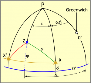
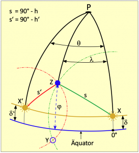
A calculation of the position is basically a simple geometry task. In Figure 4.5 all elements are present to explain the calculation path well. In it, P is the north pole, and X and X‘ are the positions of the sun or its zenith point at the times of a first and second observation. The central point Z is the zenith of an observer and thus the position of a ship.
These four points form a total of four spherical triangles. The large triangle XPX‘ outlines three smaller triangles, consisting of the two polar triangles XPZ and X’PZ, formed from a first and a later second observation of the Sun. Finally, there is the third central triangle XZX‘.

All triangles are surrounded by great circle arcs. Thus the ζ and σ angles do not end on the declination line shown in orange, because that is not a great circle. They end on the great circle arc q, the shortest connection between the solar zenith points X and X‘. The sides s and s‘ are the complements of the respective observed heights of the sun, because s = 90° – h and s‘ = 90° – h‘. It is easy to prove that these are also great circle arcs. As is well known, the shortest distance between two points on a sphere follows a great circle line. A direct line of sight to a celestial body also follows a shortest connection and this line of sight lies congruently perpendicularly above the great circle arc. The sides p, p‘ and b follow meridians and are therefore great circle arcs anyway. The side b is a common side of the two polar triangles and the complement of the position latitude The task consists first of all in calculating the arc length of the side b.

 

 

4.3.1 Calculating the latitude

The calculation is quickly done with the cosine side theorem alone. We remember its two uses:

• The cosine of a side is equal to the product of the cosines of the other two sides added by the product of the sines of these two sides multiplied by the cosine of the intermediate angle.
• The cosine of an angle is equal to the cosine of the side opposite the angle, reduced by the product of the cosines of the other sides, divided by the product of the sines of the other sides.

This now gives the following five-point plan:

1. According to A., with the sides p and p‘ of the comprehensive triangle and the angle θ enclosed by them, the side q is calculated.
2. Then all the sides of the large triangle are known, and the angle σ is determined according to B.
3. Since all sides of the central inner triangle are also known, the angle is also determined in the same way according to B.
4. From the angle difference ψ = σ – ζ one obtains the intermediate angle of the sides s and p.
5. Since the sides s and p are known and now also the angle enclosed by them , the side b can be calculated, or better the complement of this side.

So the whole thing is quite clear and we want to implement the plan formulaically right away. All we need is the cosine side theorem.

1) According to A. the equation applies to the base side of the comprehensive triangle:

   

After replacing all variables with their complements according to table 4. 1 it follows

   

and finally:

(4.3)  

2) The calculation of the angle σ is done using B.:

   

After replacing the variables with the complements it follows:

   

and finally:

(4.4)  

3) What the sides δ and δ‘ represent in the large triangle make up the sides h and h‘ in the small central triangle. The formula for calculating the angle ζ is therefore the same as Eq. 4.4, except that δ and δ‘ must be exchanged for h and h‘ and we write:

(4.5)  

4) In order to be able to calculate the side b according to A., the angle between the sides p and s must be known. This is the difference

(4.6)  

5) The side b is the complement of the latitude ψ. One could therefore formally calculate b and subtract it from 90°, from which the latitude follows. However, instead of b, it is better to calculate the complement of b, namely the latitude . For this, however, the arc sine function must be applied. We therefore write:

(4.7)  

Figure 4.5 shows that the circles of Position with radii s and s‘ intersect at two possible points and thus a position Y south of the declination latitude is also possible. This is always to be calculated if the midday sun is observed in the northern hemisphere.
If the southern intersection of the circles of Position is to be calculated because the current site latitude is south of the declination latitude, then the declinations δ and δ‘ must be multiplied by -1 before they are used in the equations. This reverses their sign and has the effect of turning the globe upside down. That is why the latitude calculated with equation 4.7 must also be multiplied by -1 at the end.

4.3.2 Calculation of the Longitude

The length is calculated analogous to the procedure in 1.4 as chronometer longitude. The applicable angle calculation according to the cosine side theorem (theorem B.) gives:

(4.8)  

Depending on whether the sun was observed in the morning or in the afternoon, the calculated hour angle must be added to or subtracted from the GHA, the local hour angle of Greenwich.

We made two observations so far, the first in the mid-morning and the second in the afternoon, as shown in Figure 4.6. However, both observations can also take place in the morning or both in the afternoon, as shown schematically in the middle and right of Figure 4.7.

Both observations are suitable for calculating the site length. We will use the first observation. If this takes place in the morning, then the culmination of the sun at the ship’s location has not yet taken place. Until then, the sun must still overcome the hour angle calculated with equation 4.8 with its constant angular velocity. The site length is thus calculated as the sum of GHA and . If the first observation takes place in the afternoon, as can be seen on the right in figure 4.7, then the longitude results from the GHA minus the calculated hour angle. Thus, the general rule is:

(4.9)  

The designation λ* is necessary because with this indication a longitude from 0° to 360° around the globe is meant. However, the geographical longitudes count from the zero meridian to 180° to the east and to -180° in the negative to the west. The negative sign for the longitudes can be omitted if the designation „W“ for west is added instead. This also applies to south latitudes if they are followed by an „S“.

The conversion from λ* to λ is done in two steps. In the first step, carryovers have to be handled. Indeed, the addition or subtraction of GHA and can produce negative results, but also values larger than 360°. In the first case, 360° must be added and in the second case 360° must be subtracted. The following example shows the necessary steps. First step – carry-over treatment:

λ* = 363° → 363° – 360° → λ* = 3°
λ* = -15° → -15° + 360° → λ* = 345°.

In the second step, a distinction is made between east and west longitudes. The rule here is that they are west longitudes as long as λ* is smaller than 180°. If λ* is greater than 180°, then λ* is to be subtracted from 360° and they are east longitudes. The examples continued finally give:

λ* = 3° → λ = -3° oder 3° W
λ* = 345° → λ = 360°- 345° = 15° E.

4.3.3 Realisation as a Computer Program

The method described above can be implemented relatively easily in a programme for determining the position at sea. The required initial values are only the data from two observations of the sun:

1. 1. • Date and time of the observations,
      • observed heights h and h‘.

In the settings of the programme it should be defined whether the sun is measured at its upper or lower limb. From the freeboard height of the boat, the eye height is also fixed as a constant. The index error of the sextant used should also be stored. From this and from the measured heights, the programme can correct the values read from the sextant. The result is the observed altitudes.
Greenwich angle and declination can either be calculated with a small module, as described at the chapter 7, or they can be taken from a stored database. Input values for this are the date of the observation and the times to the second at which the sun was placed on the horizon in the sextant’s telescope.
These data are sufficient to calculate the site width with equations 4.3 to 4.7 in one pass in succession. After calculating by means of equation 4.8, equation 4.9 then immediately gives λ*, from which, after a few reinterpretations, the longitude follows. A prior location estimate is not necessary and there are also no restrictions regarding a maximum permissible height as is usual with the standard line methods.
However, one problem has to be solved beforehand. So that the computer does not have to be told after each observation in which hemisphere the sun was observed, a mathematical way should be found for this to find out whether addition or subtraction is necessary in equation 4.9.
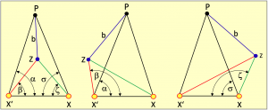
Figure 4.7 shows schematically the three possible variants of how the Sun can be observed from a position Z. The position can be west or east of the black drawn sun meridians or in between.
If it is in between, as in the left representation, then both differences α – β and σ – ζ are positive. In the middle representation the difference α – β is negative and in the right representation σ – ζ is negative. It follows that:

1. 1. 1. α – β ∧ σ – ζ > 0 
first observation east, second observation west.
      2. α – β < 0 
both observations east,
      3. σ – ζ < 0 
both observations west.

With this calculation rule, a computer programme can now work without having to enter the observation direction each time. Only in case 3. the first observation is west and then subtraction is done in equation 4.9.

The angles α and β are not normally needed. However, their calculation equations should still be given. They are:

(4.10)  

(4.11)  

Here again as a reminder: To set up these two equations only the rule mentioned under B. has to be applied, because all sides in the triangles are known.

 

4.4 Change of Location

When navigating with the sun, a reasonable time must elapse between observations so that the differences between the sun’s positions are large enough and the circles of position cross at a sufficiently large angle (>30° if possible). As sailing continues in the meantime, the ship’s location changes. If the altitude of the sun determined during the first observation can be extrapolated to the location of the second observation, then at the time of the second observation one has two suns at the same time, an imaginary sun at the position where it was during the first observation and the true sun. With this, a position can then be calculated in the same way as if one had observed two stars at the same time or immediately after each other.
This task applies to all navigation methods in which only one star is used for navigation, for Sumner and Hilaire as well as for Gauss. In these cases, the change in position between the observations, consisting of a distance over ground and a course over ground, must be determined with the aid of dead reckoning.

4.4.1 Sailing according to Douwes

Let us assume that the position of a star on the celestial sphere does not change after an observation. The star would thus maintain a geostationary state and the position of its zenith point on the Earth’s surface would also remain unchanged. If we then change our position because we continue to sail after the first observation, our distance to the zenith point would change, become larger or smaller. This distance is the radius of the circles of Position of the geostationary object on which we are always located.
At the location of the second observation, we want to determine our position by using the altitudes of the true sun and the fictitious geostationary sun. However, this is only possible if we can calculate the altitude of the fictitious sun, whose position has remained unchanged, from the distance we have sailed in the meantime and the course we have sailed, both over ground.

Figure 4.8 visualises the process as a graph. After a first observation of the sun, where its altitude was measured with h, it remains fixed in its position as a fictitious geostationary sun and thus also its zenith point BP on the earth’s surface. Now, however, we continue to sail, covering the distance from A to B on a course of c. This changes the altitude of the fictitious sun. This changes the altitude of the fictitious sun from h to hs and thus the radius of the circle of Position by Δs.
A positive change in the zenith distance is equal to a negative change in altitude Δs = -Δh). Douwes has given a formula for calculating this change in height. We do not want to derive this now, but merely state it:

   

Here d is the distance over ground (DMG = Distance Made Good) in nautical miles and c is the mean course or course over ground (CMG = Course Made Good). Because the change in altitude must be given in degrees, just like the altitude, a division by 60 NM/degrees is necessary. The letter z is the azimuth. 
The altitude of the fictitious sun after sailing is thus simply calculated as

(4.12)  

This process is called altitude adjustment after a change of location. The data of d and c needed in this formula are the results of a dead reckoning, which can be done either „on foot“ or with the help of a small programme. The azimuth z is comparable to a true heading to the zenith point. True means that the angle z is to be measured from the meridian p or p‘ pointing north. We now want to calculate the azimuth.
In figure 4.9 the azimuth to the sun X exists as the angle between the triangle sides b and s and the azimuth to the sun X‘ as the angle between b and s‘. The interior angle z* of these triangles is calculated with the cosine side theorem according to rule 2. The general formula applied to the respective measured altitude is:

(4.12)  

Since the arc cosine can only provide angles between 0° and 180° degrees (interior angle), but the azimuth ranges from 0° to 360°, azimuths that result after the ship’s noon, i.e. when the sun has overtaken the ship’s location and thus the LHA starts counting again from 0°, must be considered and possibly corrected according to the following rules:

   

   

If the LHA has 180°, then the zenith point of the sun is on the opposite side of the earth and it is deepest night. From ship’s noon until then it was always smaller than 180°. In this case, the azimuth is the exterior angle as shown in Figure 4.9 on the right.

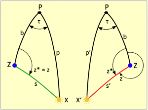
From midnight until noon, the LHA increases from 180° to 360°, i.e. it is always greater than 180°. In this case, only the interior angle of the polar triangle shown in Figure 4.9 on the left can be calculated as the azimuth and z = z*.
In the time when there were no calculating machines, an analytical consideration of a Change in location would have been out of the question. As the two formulas above show, to calculate the azimuth one needs the site width and the LHA, which is only obtained via the site length. This means no less than that the position at the location of the second observation has to be calculated once completely, without considering any Change in location. With logarithms, a fast human computer might have managed this in one hour. This does not yet take into account any Change in location. The result would only be a nearby position, which is neither the current position nor the position of the first observation. But only this fictitious position allows a very well approximated calculation of the LHA and also the azimuth. In the meantime, a dead reckoning would also have to be carried out to find out the distance and course of the location changing.
But then the second act would follow, in which the formulas used in section 4.3.1 ab 3) to calculate the sailed latitude and the following formulas to calculate the longitude would have to be calculated again. In this second run, the adjusted height hs from equation 4.12 is used instead of h. More calculation stress with logarithms is actually hardly imaginable – and that for a single mathematically exact location determination. It is therefore not surprising that approximate solutions were resorted to in the 19th century.

4.5 Position from Noon Latitude

In all methods using only the sun, there are difficulties in calculating a position from an altitude measured at or near the ship’s noon. One of the two triangles in Figure 4.5, either XPZ or X’PZ, mutates into a vertical line at noon because all sides of the triangle then coincide with the solar meridian. Thus, a position can only be derived from the noon latitude and a circle of position. This can even offer some advantages in some situations, namely when sailing near the declination latitude or very far north or south and the circles of position at these locations are either very small or very large.
The noon latitude is known to be determined by measuring the culmination altitude of the sun. Depending on whether the sun is bearing south or north, the zenith distance and declination are added or the declination is subtracted from the zenith distance. In detail, the following applies to the noon latitude:

(4.14)  

(4.15)  

When combining navigation with circles of position and noon latitude, there are two variants which are examined below.

4.5.1 Circles of Position first

In this variant, the sun is observed in the eastern hemisphere in the morning, as shown in the diagram in Fig. 4.10. The horizon distance is measured with h and, with s = 90° – h, is the radius of the circle of Position shown in the dashed line. The observation time provides the solar positions GHA and δ via an almanac.
Some time later, at noon, the culmination of the sun is determined and the noon latitude calculated. If possible, it should be determined beforehand when ship’s noon is. The most elegant way to do this is with the app described in chapter 2. It always shows the time of ship’s noon after a second observation. This second observation can be made an hour after the first observation, but still in the morning.
At noon, the ship’s own position Z is on the smallest possible circles of Position, which is shown as a red circle in the picture. However, no position can be derived from the measured culmination altitude. The polar triangle X’ZP no longer exists, it has become a line. Using δ‘, however, the noon latitude can be determined. In this case, it is also equal to the position latitude:

   

Since the first observation, however, a distance d has been travelled on a course c. The diameter or wheel has changed. This has changed the diameter or radius of the dashed circles of Position. The altitude adjustment is calculated here according to Douwes.

The azimuth used for this follows from , δ and h. Since the measurement was made in the morning, the calculated azimuth z = z* is also the true azimuth and the adjusted altitude hs can be calculated using the values of d and c.
In fact, the azimuth should have been calculated for the position of the first observation. However, this was not possible because no latitude was known at that time. In view of the great distance to the zenith point of the sun, a resulting calculation error, because the noon latitude is used, is easily negligible – as is the fact that the altitude adjustment formula is based on rules of plane trigonometry. This, too, is of no great significance for the small distances which could be sailed in one day. Much more deviations arise from the fact that the strokes sailed during a sail are not estimated and summarized up accurately enough.
The zenith distance created by the adjusted height hs is now ss and is the radius of the circle of Position shown in green in the picture. From the height hs adjusted with equation 4.12, the declination δ‘ and the noon latitude as the third element, all sides of the polar triangle XPZ are now known as complements and the angle can be determined. This then yields the site longitude λ* as the sum of and GHA:

(4.16)  

(4.17)  

Again, any carryovers must first be removed. If thereafter λ* is between 0° and 180°, then we are dealing with west longitudes. Values greater than 180° must be subtracted from 360° and are then east longitudes.

4.5.2 Noon Latitude first

In case the noon latitude is determined first, it may change due to sailing Change of location. At the time of measuring an afternoon circles of Position it is then

   

and it is the reached location latitude. Here Δ is the change in width during the sailed location change. The amount of Δ is negative if the change of location had a more southerly component, i.e. the latitude has decreased, and positive if the latitude has increased in the course of the sailing.

Figure 4.11 shows an example in which, after determining the noon latitude, sailing continued in a northerly direction. The change in width is positive here. After measuring the culmination of Sun X at noon, the Greenwich angle does not have to be determined. It is sufficient to determine the declination with the help of an almanac so that the noon latitude can be calculated from it. Since the sun was observed in the south, the noon latitude is simply 90° – h + δ.
At the time of the second observation in the afternoon, the true Sun X‘ is observed at an altitude of h‘. After taking the declination δ‘ for this time from the almanac, all three sides of the polar triangle or their complements are known. We are therefore able to calculate the hour angle . Since we have also read out the Greenwich angle GHA from the almanac, we can now also determine the longitude λ*. The formulas for this are:

(4.18)  

(4.19)  

Finally, the earth-orbiting longitude λ* must then be converted to the geographical north or south longitude.

 

4.6 The Method of Carl Friedrich Gauss

Johann Carl Friedrich Gauss was a German mathematician, statistician, astronomer, geodesist, physicist and electrical engineer. Because of his outstanding scientific achievements, he was already considered the „Princeps mathematicorum“ during his lifetime. Gauss was in charge of surveying the Kingdom of Hanover from 1821 to 1825. But he had already demonstrated his interest in land surveying much earlier.
Between 1802 and 1807 he carried out trigonometric surveys, among other things, far beyond the urban area of Brunswick.
In doing so, he used a sextant that he borrowed from his friend Franz Xaver von Zach. Using the method of least squares, which he developed himself, he was able to minimise observation errors and thus make very precise measurements.
In 1807, Gauss was appointed university professor and observatory director in Göttingen. However, the observatory was not completed until 1816. In addition to mathematics and his land surveys, astronomy was another field in which Gauss enjoyed international renown with remarkable achievements.

Gauss wasn’t a sailor, but determining the location at sea is not really different from determining the location on land. After all, a cartographer must also be able to draw lines of longitude and latitude on his maps. Thus, the dissertation of a Mr Kraft was the occasion for a remarkable work for Gauss, with which he also provided a solution to the seafarers‘ problem of two heights at the same time. In his work, W. Kraft describes how the latitude is calculated from the measured altitude of two stars.
His work was based on the model known to every astronomer at that time with the two common star positions X and X‘, the vertex Z to be determined and the north pole P, as shown in Fig. 4.13. But for the first time there was a decisive difference. Mr Kraft did not follow on the graphic model, but on a system of equations into which he had previously transformed the drawing, thus describing it mathematically exactly with two connected equations. This transformation from a generally understandable pictorial model into an abstract mathematical model was a new approach.
On the basis of a drawn thing, there is a visual contact with a problem that can be imagined more easily. Using a drawn model, it is easier to develop solutions for calculating as yet unknown elements from existing known elements. In this way, one can calculate real elements or parts of such a model step by step, trying out different solution paths until one arrives at a desired or acceptable solution. That is the way an engineer works.
Mr Kraft, however, was not an engineer but a mathematician and therefore translated the visual language conveyed by a drawing into his abstract mathematical language. He set up an equation for each of the two triangles XPZ and X’PZ. Both equations contain the latitude and the hour angle as unknowns. Thus, there is a system of equations with two unknowns. His aim was probably to shorten the calculation path, which was given with equations 4.3 to 4.7, with a analytical resolution. The system of equations is:

   

   

These two equations and Figure 4.13 are thus absolutely identical and mutually convertible into each other. The difference is only, as already mentioned, that the drawn picture corresponds to the language of the practitioner and the system of equations to that of the mathematician.
The equations, it is application of the cosine side theorem, contain the transcendental functions sine and cosine. But there is no general solution for this that could have been applied. Transcendental systems of equations are even commonly regarded as unsolvable.
Mr Kraft succeeded in calculating both the latitude and the hour angle , but in an extremely complicated resolution. Gauss remarked that it would instead be easier to find the latitude by looking directly at three triangles. This is the calculation path with equations 4.3 to 4.7. He also found peculiar Mr Kraft’s special constraint that the altitudes of the two stars would have to be measured at the same time.
This would have required two measuring tools and two observers at the same time. The sun would then even be eliminated as a navigational star because it can only have one altitude at the same time. Gauss considered the sun to be of particular importance because it shines all day long and the angle on the sextant is much easier to read in daylight.

 Gauss recognised the advantage that this new mathematical approach could mean for work in cartography and for seafarers. So he set about working out his own and better solution using Mr Kraft’s approach. The result of his work, which he did as early as 1808, appeared in „Bode’s Astronomisches Jahrbuch“ für das Jahr 1812“ under the title:

„Neue Methode, aus der Höhe zweier Sterne die Zeit und die Polhöhe zu bestimmen, nebst astr. Beobachtungen, vom Herrn Professor Gauß in Göttingen.“

The essence of this essay is contained in Article 8. It could have been a great moment in deep-sea navigation and Gauss himself was convinced that he had found a method that was finally suitable for practical applications, but he was to be mistaken.
In fact, his formula apparatus made possible a precise calculation of latitude and time. The calculation with logarithms was about a third shorter than the method with polar triangles. The calculation of time also made it possible to determine longitude.
But that was not the problem. In the end, his resolution consisted only of substitutions, which he labelled F, V, W and G, but which could not be assigned to a single element from practice or the known graphic model in Figure 4.13 or 4.5. Although it was possible to calculate latitude and time quite easily with these substitutions, and finally longitude from time, no one could develop an idea from this as to what all this was exactly. For practitioners, neither the way of analysis was comprehensible nor did the results have any recognition value. 
Gauss found a solution without using with a single formula from spherical trigonometry, which was just a new challenge for the sailors of the time. He found a solution solely by applying a mathematical analysis. Thus his method was not communicable and this is still true. It has not survived in nautical literature and is completely unknown today. I do not want to derive the formulae here, but only present them and explain how they are used. Their derivation is presented in Article 8. The formula apparatus consists of seven quite clear equations:

(4.20)  

(4.21)  

(4.22)  

(4.23)  

(4.24)  

(4.25)  

(4.26)  

Although the formulae cannot be explained in a comprehensible way, as for example with the cosine side theorem with triangular sides and angles enclosed by them, one can nevertheless calculate very well with them. Due to its symmetry (see Figure 4.3), the cosine always yields two results, one positive and one negative. This applies here to equation 4.22 for calculating W. From this, two possible positions are calculated, which Figure 4.13 shows with Z and Y north or south of the declination latitude. With the factor P in equation 4.22 it is easy to determine which position is to be calculated. With P = 1 it is the northern intersection point Z of the circles of Position and with P = -1 the southern intersection point Y.

Equation 4.24 should also be remarkable. This , which is output here via the arc tangent, is a longitude component which automatically takes the bearing direction into account. It is therefore no longer necessary to specify it, as described in section 4.3.2. A program-technical realisation therefore does without equations 4.10 and 4.11. The longitude is simply calculated as the sum of according to equation 4.24 and GHA. Furthermore, the multiplication of the declinations by -1 is omitted if the southern intersection is to be calculated, as is the case with the geometrically based solution finding in 4.3.1.
Even if the time of day of a second observation is smaller than that of a first observation, e.g. because a date change occurred when sailing through the Pacific, this is taken into account by the Gauss formulas. All in all, the formula apparatus is very compact and ideally suited for use in a computer programme.
After the altitudes and times of two observations of the Sun have been entered into such a programme, the calculation can start. In addition, the sailing data Distance d and Course c must be already available at the time of the second observation. The algorithm then runs as follows:

1. 1. 1. The programme calculates Greenwich angles and declinations from both observation times. Alternatively, these can also be taken from a database.
      2. All equations from 4.20 to 4.26 are calculated in one go. If there was a change of location in the time between the observations, the coordinates and λ* denote an unknown location in the vicinity, which is needed for an altitude adjustment after a determination of LHA for the calculation of the azimuth z.
      3. The local hour angle LHA is calculated from λ* and GHA in order to determine the azimuth z according to equation 4.13.
      4. With the azimuth and the data of sailed distance and deposed course, the adjusted altitude hs is now to be calculated according to equation 4.12.
      5. With the adjusted altitude hs the calculation is started again from equation 4.22 and all formulas up to and including equation 4.26 are run through again, whereby hs must now be used instead of h.

This means that the final position after sailing is known with longitude λs* and latitude s is fixed (index s = sailed). What is still missing is the conversion of λs* to the geographical longitude according to the usual interpretation that λs* up to 180° indicates west degrees and values beyond that, subtracted from 360°, are east degrees.

Because the Gauss formulas have never been used in shipping, they are not known to give incorrect results under certain conditions. This is the case if the declinations are not zero and additiona the heights of the sun are too small or the overlap of the position circles is too small. To avoid these errors, the following measures are necessary:

1. 1. • If the difference F – δ becomes negative, then V must be increased by π or 180°.
      • If the product of P ･(G – δ) becomes negative, τ must be increased by π or 180°.
      • If the product P･(π/2 + W – V) is negative, then G must be decreased by or 180°. If it is positive, then G should be increased by the same value.

---

Some authors wrongly attribute the method described in 4.3 to C. F. Gauss. However, this was precisely the solution Gauss wanted to avoid. After he had verbally described the geometric model shown in Figure 4.13 in his publication, he formulated the following sentence as an introduction to his way of calculation:

„All this is based on purely geometrical, admittedly quite simple considerations: however, it will no doubt be pleasant for many to see a direct solution of this problem developed in a purely analytical way, which will confirm anew that all truths that are derived from geometrical considerations can be discovered just as elegantly with the help of analysis, if this is only treated in the right way.“

So Gauss looked for a purely mathematical solution, without having to make geometric considerations about triangles, sides, angles and spherical trigonometry, and hoped that it would be simpler than the one previously known. Unfortunately, such a solution is less suitable for humans but more suitable for computers. Gauss was with it far too far ahead of his time.

The true solution found by Gauss has never appeared again in nautical literature and cannot be found anywhere in international literature either, which is a great pity, because it is precisely such solutions that are important for a digitalisation of astronavigation. Therefore, I have added a longer excerpt from his original publication of 1809 in chapter 8. This reproduction should be a treat for all mathematics fans.