links → HOME, chapter 1, chapter 2, chapter 3, chapter 4, chapter 7, chapter 8
5 Dead Reckoning
Dead reckoning means the coupling of individual route sections, so-called legs. It is carried out with the simplest of means and the evaluation is therefore quite complex. For its application, the navigator uses simple and thus reliable instruments to track three things:
- Compass direction of the boat,

- speed through the water,
- time spent on each course direction and each speed of travel.
With this information, the navigator could calculate the route and distance the boat was travelling and mark it on a nautical chart. With carefully executed dead reckoning, error rates as low as 5% are achievable. Dead reckoning used to be applied when the ship had to navigate in complicated waters at night. However, this usually only applied to warships. Merchant ships usually dropped anchor in such a case. But why do we still need dead reckoning today?
Astronomical navigation requires altitudes from at least two ncelestial bodies to determine a position, either at the same time from two different celestial bodies or from one celestial body such as the sun at different times. The line of poisition of the observed celestial bodies should not intersect at too acute an angle. When using the Hilaire intercept method, the angle of intersection should not be less than 30° so that the point of intersection of the position lines can still be read out accurately enough. After all, Hilaire’s method is a graphical one and in the past pencil lines were used, which could sometimes be thicker.
When working with computer support, the intersections are calculated and a line thickness can not have any effect. Nevertheless, even there the intersection angles must not become too acute, because then even small deviations in the observation of the horizon distance would lead to larger location deviations. To ensure an acceptable crossing angle of greater than 25°, a sufficiently long time must elapse between sun-observations.
Unless there is a dead calm, one will move away from the location of the first observation. But with every change in distance from the zenith point, the altitude at which a star is observed also changes, even if it remains mentally frozen in its geostationary position in the sky. The task now is to find a resulting course CMG, a resulting total distance over ground DMG and a resulting velocity VMG from the different courses and distances between the observations. In doing so, any current that may be present must also be taken into account, as well as any offset due to wind.
One will always want to sail courses in which the wind is optimally utilised. When sailing with half wind, the apparent wind comes in from the side. This condition allows for the highest speed. However, the boat does not sail in the direction of the keel. Rather, the bow is turned slightly into the wind. The instreaming fairway on the leeward side presses then against the slightly transverse keel and the underwater hull. In this way, a balance is established between wind pressure to leeward and dynamic water pressure to windward. However, the compass pointing in the direction of the keel no longer indicates the course. The wind also hits the freeboard area of the hull and the superstructure, which do not necessarily contribute to the balance of forces, and additionally drives the boat downwind.
Trying to judge all this correctly is an art of the skipper. You can’t really calculate all this and the effects are different for every type of boat anyway. If several tacks are sailed, this effect will even out. For example, the skipper or navigator will assume a course of 270° with a north wind and a compass reading of 280°. In this case, he has fed the compass course with -10°. Ultimately, we need the route over ground and this is not created by the boat’s propulsion alone.
Depending on the sea area, ocean currents can contribute to the speed and course being quite different from the readings of the instruments on board. For dead reckoning to be as accurate as possible, it is therefore also important to take the ocean current into account. This is taken from special current charts. However, it is better to use an ocean current radar that provides live data. Internet access is required for this. If you don’t have internet access, you can call someone via satellite phone to get the data. When using analytical navigation methods, the time span between two observations can be kept somewhat shorter because they calculate more accurately. In areas with low currents, this hardly causes any significant error. Nevertheless, it will be shown below how a coupled route is calculated taking into account ocean currents.
5.1 Two Velocities
A leg is defined in the following as a uniformly travelled distance in a certain course. This means that a new leg always starts after a tack, a jibe, a sustained change in speed or a sustained change in course. The length or distance of a beat and the course of this distance are influenced by the boat’s propulsion, but also by the strength of an ocean current.

Figure 5.1 shows the correlation. Thus, the velocity v1 generated by the boat’s propulsion takes place through the water in a flow field that drifts in a different direction at the velocity v2. The resulting velocity v is obtained by putting the two vectors v1 and v2 together.
The resulting course c on which the boat then moves is the angle between the northward direction v1 and the velocity vector v. In the picture, the eastward velocity generated by the boat’s propulsion is increased by v2λ due to the current and the northward velocity is decreased by v2.
5.2 Addition of the Legs
The respective distances are the products of velocity v and duration t. Since only the sum of all north-south sections and the sum of all east-west sections are needed for an overall assessment, no matter how many turns or jibes were made, these must first be defined. With the counting index i for each leg, i.e. i = 1 to n, if n beats have been driven, the following apply initially:
(5.1) ![\[\Delta\varphi_i=t_i\,(\text{v}_{Ai}\cos c_{Ai}+\text{v}_{ci}\cos c_{ci}),\]](https://astro-navigation.com/wp-content/ql-cache/quicklatex.com-16ced7c9aa9131983b2905d13ef0ae7b_l3.png "Rendered by QuickLaTeX.com")
(5.2) ![\[\Delta\lambda_i=t_i\,(\text{v}_{Ai}\sin c_{Ai}+\text{v}_{ci}\sin c_{ci})\cdot\]](https://astro-navigation.com/wp-content/ql-cache/quicklatex.com-947f60e33442248f775af6f423431355_l3.png "Rendered by QuickLaTeX.com")
Herein apply to each individual beat:
- i No. of the driven stroke
- Δi North-South component
- Δλi East-West component
- ti Time duration in hours
- vAi Course through water in degrees
- cAi Propulsion speed
- vCi Current velocity
- cCi Direction of flow
The sections according to equations 5.1 and 5.2 are now added up separately for each leg and the total distances covered in the north-south and east-west directions are obtained.
The total north-south distance covered is then written:
![\[\Delta\varphi_T=\Delta\varphi_1+\Delta\varphi_2+\Delta\varphi_3+ ...\Delta\varphi_n =\sum_{i=1}^n \varphi_i\cdot\]](https://astro-navigation.com/wp-content/ql-cache/quicklatex.com-8d6894126317a3de39f7fb1d31f3e69f_l3.png "Rendered by QuickLaTeX.com")
For the total east-west intercept, the same:
![\[\Delta\lambda_T=\Delta\lambda_1+\Delta\lambda_2+\Delta\lambda_3+ ...\Delta\lambda_n =\sum_{i=1}^n \lambda_i\cdot\]](https://astro-navigation.com/wp-content/ql-cache/quicklatex.com-044f7d7e53dd9c0b6c49108b885a2f03_l3.png "Rendered by QuickLaTeX.com")
Geometrically, these distances form a right triangle as shown in the top half of Figure 5.2 for the first quadrant. The catheens are the sums of all north-south and east-west components of the triangle. The total distance travelled over ground d (DMG) is simply calculated from this using the Pythagorean theorem:

![\[\text{d}^\circ=\sqrt{(\Delta \varphi_T )^2+(\Delta \lambda_T )^2}\]](https://astro-navigation.com/wp-content/ql-cache/quicklatex.com-71bd8cae18310f3d950a7be2d4a29a28_l3.png "Rendered by QuickLaTeX.com")
However, the course c (CMG) travelled in the process is also entered in the picture. In a right triangle, the tangent of an angle is calculated as the quotient of the opposite and opposite sides. We thus obtain:
![\[\tan(90^\circ-c)=\frac{\Delta\varphi_T}{\Delta\lambda_T}\]](https://astro-navigation.com/wp-content/ql-cache/quicklatex.com-0711bdba9c6fb1d6eaf90f9851f6f266_l3.png "Rendered by QuickLaTeX.com")
The arc tangent function directly gives the angle, i.e. 90° – c, and we get
![\[90^\circ-c=\arctan\frac{\Delta\varphi_T}{\Delta\lambda_T}\]](https://astro-navigation.com/wp-content/ql-cache/quicklatex.com-96838152e0f506a9c8c339bc193cb6e5_l3.png "Rendered by QuickLaTeX.com")
and finally
![\[c=90^\circ-\arctan\frac{\Delta\varphi_T}{\Delta\lambda_T}\]](https://astro-navigation.com/wp-content/ql-cache/quicklatex.com-714289ebabb88637181ce108e9e0a2e7_l3.png "Rendered by QuickLaTeX.com")
In the second quadrant, the angle between a circle of latitude and the singeing vector, we call it α for now, is calculated with
![\[\alpha=\arctan\frac{\Delta\varphi_T}{\Delta\lambda_T}\]](https://astro-navigation.com/wp-content/ql-cache/quicklatex.com-c94fe663f72641dbb80c5a4d010bee0a_l3.png "Rendered by QuickLaTeX.com")
In the second quadrant, the sum of all latitude changes is negative and the course is southeasterly. Thus the arc tangent is also negative and the addition in the above equation becomes a subtraction. For this reason, the same calculation formula applies to quadrants 1 and 2 and this is the upper one in equation 5.4. It applies to courses with an easterly component. Since α is the angle between the circle of latitude and the vee, this angle α is entered as c – 90° in the lower part of figure 5.2.
(5.4) 
The same considerations can now be made for courses with western components. It will then be seen that the arc tangent must now be subtracted from 270° as indicated by the lower formula in equation 5.4. The auxiliary angles in the picture are then 270° – c and c – 270°.
5.3 The Coupling Board
This is a Aids on which the helmsman enters course, and speed with the associated time for each leg travelled. After each significant change in course or speed, a new row is created. A track can then be constructed on a map from these entries, whereby the current position is always known, even between observations. A linkage board created by the navigation app in Chapter 2 can be seen in Figure 2.16.
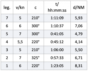
Finally, an example will show how the available numbers are processed. The following table contains seven rows, each with a leg to be processed. The difference between leg 3 and 4 is a course correction, for example, to be able to use the wind more optimally. The entry of a leg 6 on a constant course was necessary because the speed had permanently dropped by 1 kn. The following table contains all the values entered for a trip lasting more than seven hours.
You can see that a total of four tacks were made. A distance of 42.45 NM was covered through the water in the legs completed, which is the sum of the individual distances given in the last column.
The distance over ground DMG, the average course CMG and the resulting speed VMG must now be determined. Table 5.2 lists the change in latitudes and longitudes for each leg according to equations 5.1 and 5.2.
Possible ozean-currents are not taken into account in this example. From this, the DMG can now be calculated with equation 5.3 and we write

![\[d=\sqrt{8,01^2+27,84^2}=\underline{\underline{28,97 NM}}\cdot\]](https://astro-navigation.com/wp-content/ql-cache/quicklatex.com-214b38f886512d6af91b697b9baaa8ab_l3.png "Rendered by QuickLaTeX.com")
The λ-column has a negative result in the sum, so the mean course CMG must be calculated with the lower formula in equation 5.4. The result is therefore:
![\[c=270^\circ-\arctan\frac{-8,01}{-24,84}= \underline{\underline{254^\circ}}\cdot\]](https://astro-navigation.com/wp-content/ql-cache/quicklatex.com-f5b49d567d833a2c2262a8920139ae19_l3.png "Rendered by QuickLaTeX.com")
The everage speed VMG is the quotient of the well made distance d and the total time of the trip of 7:14:41 h and we get:
![\[\overline{\text{v}} =\frac{28,97\; NM}{7,245\;h}=\underline{\underline{4\;kn }}\cdot\]](https://astro-navigation.com/wp-content/ql-cache/quicklatex.com-3cc2a7ec7c5a7244998c5e01997fe35a_l3.png "Rendered by QuickLaTeX.com")
The result of the cruise is summarised as follows:
- Duration of the trip 7:14:41 h
- Trip through the water 42,45 NM
- DMG = 28.97 NM
- CMG = 254
- VMG = 4 kn
Figure 5.3 shows the individual strokes in a graph.
The app recalculates, displays and saves the results listed in 3. to 5. every minute. The current sailing data is therefore available immediately after every second observation, i.e. to the minute. Possibly existing flow data are only recorded by equations 5.1 and 5.2 as long as they are visibly entered in the input fields.

In practice, dead reckoning has only ever been carried out graphically. It would also be rather time-consuming to always try to calculate a sailed distanz with equations 5.1 to 5.4. Often the distance sailed was only estimated. However, if a cleanly working navigation programme is to be created, then one will have to go the algebraischen way shown here. For this reason, the formulas and their derivation are described here.
6 Great Circle Calculation
For small distances, the skipper will usually choose a direct course. On a 2-D chart, this is a straight line from A to B. Such a course follows a so-called rhumb line. Here the meridians, which on a 2-D chart are the vertical lines, are always intersected at the same angle. Since on a globe the distance between the meridians becomes ever narrower towards the poles, such a course, if followed long enough, has a spiral shape all the way to the pole. In principle, a path covered from A to B is not optimally short, because the shortest connection between two points on a spherical surface is along a great circle. It was Pedro Nunes who was the first to carry out investigations in this direction in 1550.

A long time ago, when it was not yet possible to determine the longitude, one first sailed along a known coast to the north or south until the desired latitude was reached, and only then began the crossing to the west or east. In doing so, one did not leave the latitude, which was regularly ensured by determining the noon or north star latitude.
Such a course is not optimally short either, for it is along a circle of latitude and a circle of latitude cannot be the shortest connection between two points on a spherical surface. The shortest connection between two points on the globe is always along a great circle line, because this has its centre at the centre of the sphere. A distance travelled on a great circle is called an orthodrome. In Figure 6.1, an orthodrome is the connection from A to B shown in green.
It is a matter of economy that the fastest and most direct course is always followed if possible. This takes less time and as the number of steamships increased, it also saved a lot of fuel. Some people may have wondered why planes take such a wide turn on long-distance flights and do not fly directly to their destination. They follow an orthodrome and on a sphere that is always the shortest and most direct route.
As a skipper, you also want to reach your destination by the shortest route on long distances and that is why we want to briefly discuss this here. You can do a lot of calculations in this regard, but I think that it should be enough to be able to determine your initial course and that you know how long a shortest route from A to B is. An end course can also be determined mathematically. But what would be the point here? It is better to repeat the initial course determination from time to time on the way. With the app presented in chapter 2, this works effortlessly.
The calculations are done with the help of the cosine side theorem. The meridian sections PA and PB shown in Figure 6.1 are known, as is the polar angle λB – λA enclosed by them, because the positions of the position and the destination are known. From this, the distance d can then be easily calculated. By using the complements A for PA and B for PB, sine turns into cosine and vice versa. Then the following applies to the distance:
(6.1) ![\[\text{d}^\circ=\arccos\big[\sin\varphi_A\sin\varphi_B+\cos\varphi_A\cos\varphi_B\cos(\lambda_B-\lambda_A)\big]\cdot\]](https://astro-navigation.com/wp-content/ql-cache/quicklatex.com-cbb4760d639492798938e065127e7654_l3.png "Rendered by QuickLaTeX.com")
Now all the sides of the triangle are known and so every angle in the triangle can be calculated. The initial course c is calculated as follows:
(6.2) ![\[c^\ast=\arccos\frac{\sin\varphi_B-\sin\varphi_A\cos d}{\cos\varphi_A\sin d},\]](https://astro-navigation.com/wp-content/ql-cache/quicklatex.com-6af325acca94b09a06f57027d1921a20_l3.png "Rendered by QuickLaTeX.com")
(6.3) 
Die Zusatzformel 6.3 regelt einen Unterschied zwischen Ost- und Westkurs. Bei einem Ostkurs ist der Anfangskurs gleich c*. Bei einem Westkurs muss c* von 360° subtrahiert werden, um den Anfangskurs zu erhalten.
Additional formula 6.3 governs a difference between eastbound and westbound rates. For an east course, the initial rate is equal to c*. For a west course, c* must be subtracted from 360° to obtain the initial course.
Finally, here is an example. A boat intends to cover the shortest distance from Charleston (NC) 32.73° N / 79.83° W and Lisbon 38.64° N / 9.31° W.
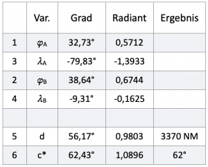
Table 6.1 contains all numerical values. Lines 1 to 4 contain the coordinates of the starting point and destination. The results of the calculation are in lines 5 and 6. The values are given in degrees and radians. Programs on computers and also spreadsheets calculate with angles in radians, which are given here in the Radian column. Reminder: 360° = 2
The arc d is an angle inside the Earth with a magnitude of 56.17° as shown in Figure 4.1 on the right. Since one degree on the Earth’s surface spans an arc length of 60 nautical miles, the arc length of d is the product of 56.17° ⋅ 60 NM/degree and thus becomes 3370 NM.