1 A brief excursion into the history of astronavigation

links → HOME, chapter 2, chapter 3, chapter 4, chapter 5 and 6, chapter 7, chapter 8

In order to determine the latitude circle on which a ship is currently located, man developed numerous tools with which he could observe those celestial bodies that gave him information about it. The most important were Jacob’s staff, quadrant, octant and finally the sextant. It has been known for a long time that the altitude of the North Star in the northern hemisphere corresponds fairly well with the latitude of the own location, and since the Middle Ages there have been reasonably useful declination tables that make it possible to determine the latitude of the own location with the culmination of the sun at noon. From this, a special navigation method developed early on, which was called „Breiteln“ in German and meant to keep stubbornly to a constant latitude.

Columbus also used this method to get back to Europe. Coming from the Caribbean, he initially sailed only northeast until he reached the desired latitude of Cape St. Vincent in Portugal, and then changed his course directly east. On his onward journey, he tried to navigate in such a way that the altitude of the North Star remained the same as far as possible, even if storms sometimes drove him off. In the course of his journey, he hit the Azores and eventually even reached Lisbon pretty much by accident.
Determining longitude, on the other hand, was considered impossible for a long time, although ways to do so had already been thought of. In the 16th century, Galileo and others were of the opinion that the degree of longitude could be determined with an exactly running clock. But the attempt to determine longitude with a pendulum clock on board only lasted until the first storm, which threw the pendulum completely out of sync and after which the clock could then no longer be set.
Later, the Greenwich Time was determined by measuring the distances of the moon to fixed stars. At the latest, this gave mathematics an important role in navigation practice.

 

1.1 The Problem of the Two Altitudes

The Portuguese Pedro Nunes (1502-1578) described a principle according to which the geographical latitude could be determined from two different altitudes of the sun. The Danish astronomer Tycho Brahe (1546-1601) is known to have been able to deduce the unknown position of a star from the known position of two other stars. Strictly speaking, this task is no different from determining the unknown position of a ship. The Earth’s grid of degrees is a projection of the grid of degrees on the celestial sphere. Thus, the position of the zenith Z of a ship on the degree grid of the celestial sphere is identical with the position of the ship on the degree grid of the Earth.

In this way, the astronomers‘ activity could be transferred to a position determination on the sea. The task would only be to derive the unknown zenith of a ship’s position from the position of two known celestial bodies or the position of the sun at two different times. This task has become known as the problem of the two heights or simply as the two-height problem.
However, a simple calculation method could not be found for this task. Mathematics was still growing. Although there were already enough work results on spherical trigonometry, they were still completely unorganized and thus not ripe for general use. A prize advertisement published by the Paris Academy of Sciences on 17 May 1727 gave a boost to the solution of the problem of two heights. A prize was to be awarded to the person who could offer a practicable solution to the problem of two heights. Among the numerous participants hoping to win a prize was Daniel Bernoulli, who is known today primarily as the founder of fluid mechanics. He wanted to determine the latitude from three successively measured heights and the corresponding intermediate times on one and the same celestial body without knowing its coordinates.
The search for simple solutions dragged on quite unsuccessfully until almost the middle of the 19th century. Countless publications of more or less practical use became known. In many cases, attempts were made to circumvent spherical trigonometry by searching for alternative solutions in plane trigonometry or even in general arithmetic instead.
In the second half of the 18th century, Leonhard Euler (1707-1783) systematized the theorems of spherical trigonometry and also gave easy-to-understand instructions on how to apply them. Because at that time the calculation was only possible with the help of logarithms, Euler even published the formulae in two variants. In the first variant, they were interpreted in their most illustrative form known today. The second variant was a so-called derived equation, which consisted only of products and quotients, and was thus optimized with regard to a computational application with logarithms. With this work, Euler had created the basis for a mathematically rigorous procedure for calculating the latitude of a location from the measured heights of two celestial bodies.

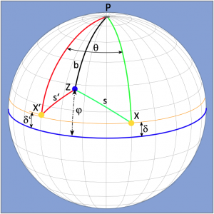
In the following, the mathematical background of the solution of the two-height problem should be explained. For this purpose, we use the sketch in Figure 1.3. In it we find the zenithal points of the sun, which are labelled X and X‘. These are the geographical positions on earth where the sun is currently at its zenith at the exact moment when its respective altitude above the horizon is measured from a location Z with a sextant. The geographical latitude of these zenith points at the times of measurement must of course be known. For this purpose, there were already tables at that time from which the declinations δ for each hour of a year could be taken. The observation times should be a few hours of solar transit time apart and, in addition, it was convenient to make the first observation in the mid-morning and the second in the mid-afternoon. A fourth reference point in this model is the pole P, which in our case is the North Pole. The connecting lines of the points XP and X’P are known and are calculated as 90° – δ and 90° – δ‘ respectively. The connecting lines of points XZ and XZ‘ are also known, because these are the zenith distances s of the measured heights of the sun, namely s = 90° – h and s‘ = 90° – h‘, where h and h‘ are the measured horizon distances. The zenith distances are also called complements of the measured horizon distances of the sun, because they are their supplements to 90°.
This results in two spherical polar triangles lying next to each other. These have a common side, namely side b. If it were now possible to calculate this side b, then one would also have the latitude of one’s own location, because here too = 90° – b applies. Mathematicians already knew the exact way to calculate the width in the 18th century. This was done with the help of the great triangle XPX‘ and the intermediate time of the solar observations, which provides the polar angle θ.
Thus, a method was known to calculate the side b and the latitude exactly from this constellation. But the computational effort for this was far too high. A latitude calculation would have taken a lot of time on board a ship, in which the ship would travel long distances. So, the method did not catch on with the seafarers. Disappointingly, the further development of mathematics did not initially bring a practical solution.

1.2 Cornelis Douwes

The astronomical task of finding the latitude of a location was considered one of the most important tasks in geography and navigation at that time. If the latitude of a ship’s location was known, the time could be determined from measured distances between the moon and known fixed stars, and from this the geographical longitude and finally the location. The lunar distance method was not entirely trivial, however, and required some calculations as well as extensive tables of numbers. Until then, the latitude could only be found by observing the North Star or as midday latitude with possible subsequent dead reckoning.
The Dutchman Cornelis Douwes (1712-1773) was director of the maritime school in Amsterdam. His vision was to make the two-height problem useful to mariners. To this end, he developed a method of finding the latitude of a location from two altitudes of the sun observed outside the noon circle. His approach was to shorten the tedious logarithmic calculation of polar triangles by creating a special logarithmic table of his own. Using this Douw’s table required less calculation and less searching in tables. A total of nine table accesses were required for a latitude calculation. This reduced the calculation effort to about one third compared to the strict calculation method with more than 20 necessary table accesses, whereby an interpolation was always necessary after each table access. His method was not entirely exact and contained simplifications. One of them was the need to guess a position in advance and the consequence of this is that instead of the position, only a better guess-location is identified.
Douwes received a handsome prize for his table method from the British Longitude Commission. Afterwards, his method became established among both Dutch and English seafarers and was a common standard method until the 19th century.

 

1.3 Chevalier de Borda

The Frenchman Jean-Borda had an extraordinarily interesting idea for determining latitude on his voyage in 1771/72, which took him along the West African coast with the exploration ship Flora. However, exact results could only be obtained by means of so-called rigorous calculations.
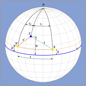
Borda made two observations of the sun in order to be able to determine its heights h above the horizon, the horizon distance. The principle is shown in Figure 1.4. The first measurement was made in the mid-morning and yielded the zenith distance s = 90° – h marked in green. The second observation in the mid-afternoon then showed the zenith distance s‘ = 90° – h‘ marked in red in the picture.
The method is particularly suitable when the latitude changes rapidly as a result of a north-south course or when the noon latitude cannot be determined because of noon sun being covered. In addition to the altitude measurements, the intermediate time t, the time between observations, also had to be recorded, but this could be measured with a simple ship’s clock.
Before starting a calculation, one’s latitude still had to be guessed. From this guessed latitude, the complements s and s‘ of the respective observed altitudes and the declinations of the observations, the hour angles ₁ and ₂ of the two polar triangles XPZ and X’PZ were then calculated. 
These were added and their sum divided by the Sun’s angular velocity of 15°/hr. The result of this was the calculated transit time of the Sun between observations. This would agree with the measured intermediate time t if the latitude had been estimated correctly.
It is easy to see from the figure that the distance between the zenith points of the suns X and X‘ increases when a smaller latitude is used because the lengths of s and s‘ remain the same. As a result, a running time of the sun would then be calculated that is larger than the measured true intermediate time t.
Now the whole thing could be repeated with a new latitude each time until it fits. However, the astronomer Jerome Lalande then had the idea of finding the probably correct latitude from two latitude estimates using a rule of three. The method proved to be remarkably accurate if the latitudes could be estimated fairly accurately beforehand. If this was not the case, then larger deviations resulted, which urged the repetition of the entire calculations. The longitude was obtained from the time, which at that time could only be determined from lunar distances to known fixed stars. This method, too, sometimes required a huge amount of calculation, and so it was not accepted by the sailors.

I was interested in the method and so I developed a program for it that even did without latitude estimation.
In the northern hemisphere, all whole degree latitudes are first checked starting from the maximum possible latitude s_min + δ and counting downwards until a valid range between two latitudes is found. This is the case when, of two consecutive latitudes, one latitude yields a time from the hour angles that is less than the measured intermediate time t, and hour angles follow from the following latitude that yield a solar transit time greater than the measured intermediate time t. The program then switches from degrees to minutes of arc and searches the area between the latitudes found in mile steps until two latitudes are found again – this time in minutes of arc precision – between which the location must lie.
I tested the program at sea and found that it can indeed find the latitude of the location to within one nautical mile. The calculations involved are simple but extensive, my smartphone didn’t mind. The result was displayed immediately after the last altitude entry. What was surprisingly new for me was the experience that positions at sea can also be found precisely without any lines of position.

 

1.4 The Longitude by Chronometer

Towards the end of the 18th century, several methods for determining latitude were already known. The most accurate was the determination of the noon latitude. The procedure required for this was carried out daily on all seagoing ships. The current latitude then had to be found by coupling. For this purpose, the latitude component that could be calculated since the last location determination by means of log and compass is added.

Without the possibility of determining longitude, it was common for ships to sail along a coast in known waters for weeks until the desired latitude was reached. Only then could they venture a passage along the circle of latitude to a known port on the other side of an ocean. During the crossing, the latitude had to be constantly determined and the course corrected if necessary.
The search for a method to determine longitude took a total of 400 years. In 1600, the Spanish king set a prize money for a way to determine it, but he was unsuccessful. More than a hundred years later, in 1714, the English Parliament followed suit and offered up to 20,000 pounds in prize money for a workable solution to the longitude problem. The occasion was the sinking of four ships that broke up on the cliffs of the Skilly Islands seven years earlier, killing about 1500 sailors.
It was not until ten years later that John Harrison took up the task. He was actually a carpenter, but had already built a clock with wooden gears. He could not let go of the vision of building an accurate ship’s clock. At that time, there were already methods for deriving the time from the occultation of Jupiter’s moons or from the distance of the Earth’s moon from known fixed stars, but the former was far too rare and could therefore only be used in observatories on land for time corrections. Lunar distance measurements, on the other hand, had already become more common on board, but were still quite complex.

With a first clock specimen from Harrison, which was later called H1, a test run succeeded in confirming the accuracy of the method. However, the prize money was not paid because the test journey did not quite meet the requirements. It could also have all been a coincidence, some critics said. In addition, there was resistance and doubters. For example, the reliability of a technical instrument was fundamentally doubted.
One permanent opponent in particular was the court astronomer of the English royal house, Nevil Maskelyne. He relied on the moon distance method because it was independent of technical instruments. Moreover, he saw the development of the longitude clock as competition to his own ideas, with which he wanted to perfect the moon distance method.
It was not until James Cook returned from his second voyage around the world in 1775 and confirmed the good quality of a model of a Harrison chronometer, today designated K1, that the longitude problem was also considered solved in astronomical circles. Harrison was awarded £10 000 in prize money. The K1 was an exact replica of the H4. A further development, now called the H5, was tested by King George III himself. The test was successful and Harrison was awarded a further £8 750.
After the H5, which cost around £500 at the time, watchmakers replicated the models and prices fell. The first mass-produced marine chronometers were available from about 1790. The fact that the Beagle had 22 of them on board during its voyage of exploration with the famous Charles Darwin shows the importance that was attached to it. It was not until the end of the 19th century that the demand for chronometers could be met to some extent – in England even earlier.

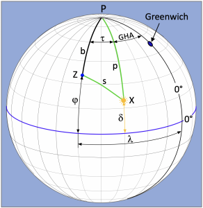
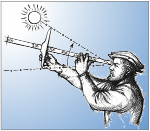
The determination of the chronometer length is a simple process, which we will now illustrate using the model shown in Figure 1.6. After the latitude has been determined, e.g. as noon latitude or DR latitude, the height of the sun above the visible horizon is measured with a sextant. After correcting the angle of altitude read off, the observed altitude h is given. The complement of this altitude, its difference from 90°, is the zenith distance s, which is drawn in the picture as the green triangular side between Z and X. The most important thing in altitude measurements is to determine the time to the second at which the star was placed on the horizon in the sextant’s telescope.
The next step is to find the declination δ from a nautical almanac. For this you also need the observation time, but only to the minute, because the declination changes only very slowly. Thus, all sides of the nautical triangle or pole triangle in Figure 1.6 are known. We now have:

Side p = 90° – δ
Side s = 90° – h,
Side b = 90° – .

If all sides of a spherical triangle are known, then each of the three possible angles in the corners can be calculated. In our case, the polar angle is calculated.
The length λ, as can be seen in the picture, consists of the sum of and a second angle designated GHA. GHA is the abbreviation for Greenwich Hour Angle. This hour angle describes the difference between the prime meridian running through the Greenwich Observatory and the meridian on which the sun’s image point is located at a time to be specified. This time must be known to the second, because the angular velocity of the sun is very high at 15°/h.  At the equator, this results in 463 m/s.
The fact that the prime meridian should pass through the observatory at Greenwich was decided in 1884 at the International Meridian Conference in Chicago. There were several proposals, including one from France, to have the prime meridian pass through Paris. Because at that time the greater amount of existing nautical literature and also numerical tables took the prime meridian through Greenwich into account, the decision fell on this place.
But now back to the matter at hand. From the constant angular velocity of the sun of 15°/h, the GHA could now be calculated if the time at which the sun passes the prime meridian were known. However, there was a problem.
A chronometer goes absolutely evenly. If it turns its 24 hours 365 times a year, then it only happens on four days that the sun culminates exactly at 12:00:00 GMT (Greenwich Mean Time), on the prime meridian. On all other days, the sun culminates before 12:00:00 or after.  Solar time and chronometer time are not synchronized. This was already suspected in the Middle Ages, and it turned out that the first pendulum clocks were not in sync with the sundials that were mounted everywhere on the walls of churches and town halls. They apparently went ahead once and then behind again – and that up to a quarter of an hour.
If the sun is to be used for navigation, then solar time must also be available. In order to obtain solar time from chronometer time, a compensation time was needed. The name for this is equation of time. So, this is not an equation in the mathematical sense, but a value from a table that provides the time compensation for a certain date. It is actually up to 16 minutes that a chronometer can go ahead or behind solar time within a year.
Once Johannes Keppler had accurately calculated the Earth’s orbit around the Sun, it was also possible to determine the equation of time. This work was carried out by the first court astronomer of the English royal family, John Flamsteed (1646-1719).

After that, the time given by evenly going so-called wheel clocks was called mean time. The true solar time, which makes navigation with the sun possible in the first place, is the sum of chronometer time, which corresponds to GMT or universal time UTC, and the equation of time. Therefore, in addition to an accurate chronometer, a year table with the equation of time must always be available on board the ships.

To come now to the determination of the GHA, imagine that on a ship in the Atlantic the culmination of the sun was observed at 14:00:00 GMT. According to the equation of time, however, the sun has already passed the prime meridian at 11:58 GMT and is therefore already 2° west of Greenwich at 12:00 GMT. It is then clear that at 14:00 GMT the ship is also not at 30° W, but at 32° west longitude.
Thus, to determine the longitude, the difference between observation time and 12:00:00 GMT must first be calculated. Then the equation of time is added and the sum obtained is multiplied by the angular velocity of the sun of 15°/h. Since the middle of the 19th century, the GHA has been tabulated in nautical almanacs, making the work with equation of time tables unnecessary. Figure 1.6 shows the case where the sun is observed from the ship in the east, i.e. in the morning. This calculates the site length as the sum of GHA and . As soon as the sun has overtaken the ships meridian, i.e. X is west of Z, the location length must be calculated as the difference between GHA and .

 

1.5 Carl Friedrich Gauß

Gauss was probably the greatest mathematician of all time. In connection with one of his favorite occupations of land surveying and cartography, he also dealt with the determination of latitude and longitude. He wrote a remarkable work on this, which was never mentioned again in nautical literature after its publication in 1812. It is noteworthy that the popular mathematician and book author Heinrich Dörrie (1873-1955) presented a method as the Gauss method in his reference book on trigonometry under the heading „Gauss und das Zweihöhenproblem“, which did not originate from Gauss at all. Several authors then further spread this misinterpretation and thus reinterpreted the true Gauss method. So what does the Gauss method really consist of? The most essential part of his original publication is therefore reproduced in the appendix of this book.
Even though Gauss was not a sailor, astronomy and cartography were only two fields among many, in addition to mathematics, in which he made extraordinary achievements. The most famous of these is probably the bell curve of the statistical normal distribution that he discovered. Other important works are the Gaussian algorithm for solving algebraic systems of equations, named after him, or the method of least squares, with which he was able to calculate the orbit of the dwarf planet Ceres, for example, so that it could be found again after it appeared to have disappeared behind the sun one day.
As a cartographer, Gauss also had to be able to determine longitude and latitude so that he could enter them on the maps. So this was not just a task for seafarers. He was well aware of the problem of the two altitudes and the calculation of latitude via the two polar triangles as shown in Figure 1.3. To solve this problem, individual elements of the graphic model have to be calculated piece by piece using formulas from spherical trigonometry, until finally the distance b can be determined, the supplement of which to 90° provides the latitude sought.
However, this task should also be solvable in a different way. For example, the graphic shown in Figure 1.3 can also be seen abstractly by not drawing the two triangles but expressing each of them by a mathematical equation. The equations are related via their common side b and an hour angle. This is then a system of equations with the two unknowns b and the hour angle existing between X and the location Z. A mathematician named Kraft first had this idea. However, his solution was very entangled and unsatisfactory and Gauss means that a solution using spherical trigonometry via the triangles would be much easier as the solution of Mr Kraft.

The system of equations consists without exception of the transcendental functions of the sine and cosine and there is no algorithm or general way to be able to solve this problem at all. Gauss, however, felt challenged and nevertheless found a way. After using the known positions of two fixed stars in a calculation example, he obtained the complete location as a result, consisting of longitude and latitude.
One problem with his method was that the calculation method was not communicable. The mathematical analysis he used was a special path that had come about as a result of a scientific dispute with Mr Kraft. So this was high-level mathematics that no sailor could have worked with. Even if it had been done, the effort compared to a trigonometric calculation via the triangles would not have been decisively smaller.
Today, almost 200 years later, we have computers, and they don’t care whether the formulae are understood by humans or not. They only have to be correct. Packaged in a computer programme, the Gauss method is an ideal navigation module. This is exactly the way it has been used in satellite navigation.
The true Gauss method was never used in navigation and is forgotten today. Gauss was far too far ahead of his time.

 

1.6 Die Industrielle Revolution

It began in the second half of the 18th century and gathered pace in the 19th century. Technology, productivity and science accelerated. Sea power and sea trade grew at an unprecedented rate. Sailing ships had to give way to the new steamships. For the industrial nations, the colonies were far away and a constantly growing population in Europe and the United States of America wanted to be supplied. The increasing shipping traffic on the world’s oceans suffered greatly from the fact that the possibilities of safe ocean navigation were still quite modest. Apart from the option of navigation by means of noon or north star latitude and determination of chronometer longitude, only Douwes‘ method was available for latitude determination outside noon. The manufacturers of chronometers tried hard to satisfy the huge demand of shipowners and captains.

To save time and thus money, the ships had to become faster. The legendary clippers, for example, achieved etmales of more than 400 nautical miles in good winds. These ships could thus run at top speeds of more than 20 knots. Despite enormous improvements in the techniques and loading capabilities of the clippers, they still could not compete with steamships in the end. However, steamships consume fuel, which costs money. If less coal has to be bunkered, then more payload can be transported. The courses sailed were optimized. But they also had to be kept to, which was only possible if the captains had the appropriate navigation facilities at their disposal.

The pressure to finally develop better navigation methods grew. Science had known exact solutions for a long time, but the computational effort required for this could not be made on board the ever-faster ships. The only calculating aids available were logarithm tables, with them had taken far too long to calculate the position. Moreover, there were not enough mathematicians to crew the fleets. In this situation, the practitioners took the matters. The American merchant captain Thomas H. Sumner is considered the inventor of the line of position and thus founded the graphic navigation methods. Three decades later, the French frigate captain Marcq Saint Hilaire succeeded in decisively improving the standing line method. The spread of the graphic methods is considered a turning point in ocean navigation as well as the beginning of the era of modern astronavigation, which only came to an end with the introduction of satellite navigation.

 

1.7 Thomas Sumner

Thomas Hubbard Sumner was born in Boston, Massachusetts in 1807, the son of an architect. At the age of 15, he began studying at Harvard University, graduating four years later. In 1829, he signed on as a seaman on a merchant ship on the China Route. Eight years later he was a captain with his own ship. Sumner was well educated and had extensive knowledge of mathematics and astronomy.
On the morning of 17 December 1837, Captain Sumner, having been at sea from South Carolina for 22 days, approached the St George Channel between Ireland and Wales. His journey was to Greenock in Scotland. It was storming and the sky was overcast. He now urgently needed assurance that the wind from SSE had not moved him too far up the dangerously flat and rocky south-east coast of Ireland. At about 10:15 the cloud cover suddenly broke and the sun became visible. This was just enough for a measurement of the Sun’s horizon distance.
The methods for determining noon latitude and chronometer longitude had been well established on many seagoing vessels since the beginning of the 19th century. However, it is not possible to determine longitude at noon with these methods. At its culmination altitude, the sun describes a very shallow arc, covering more than 100 miles to the west, without any change in altitude being detected. If the sun’s altitude is measured two hours before or after ship’s noon, then a longitude calculation based on a present latitude would only cause a small error.

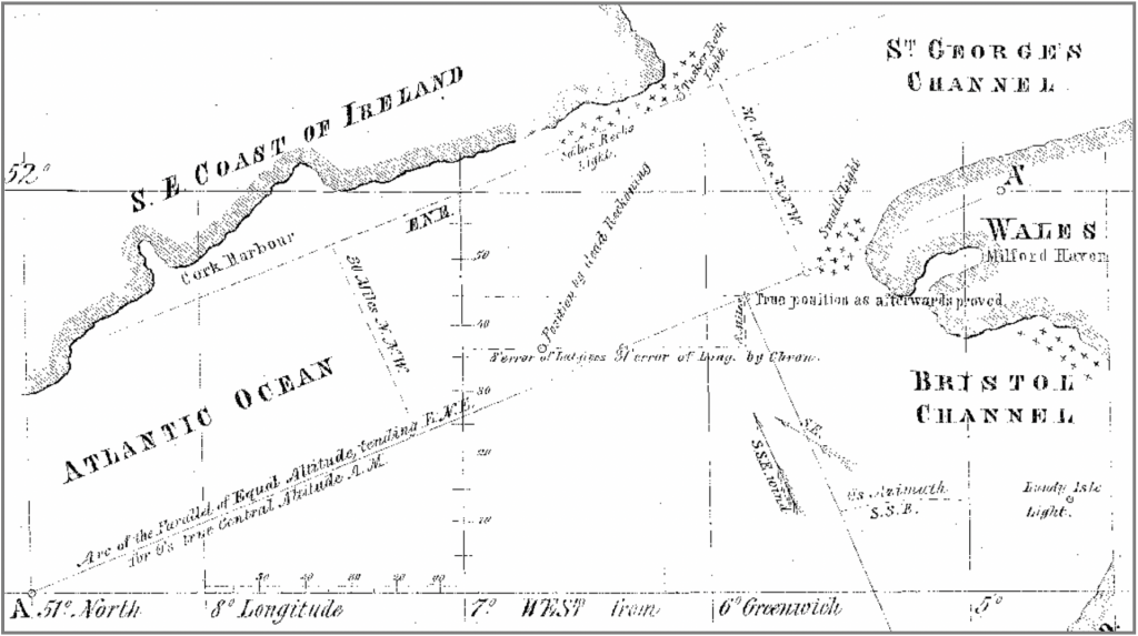
Captain Sumner was aware of this. It was therefore very fortunate that he was able to measure the altitude of the sun two hours before the ship’s noon. He was worried about his position because the strong winds could have driven him towards the Irish leeward coast. His course at that time was east-northeast and he only had an older dead reckoning position. From the measured altitude and the dead reckoning latitude he could now calculate a chronometer longitude and hence a position. The was then even east of his dead reckoning position and thus further and safer from the Irish coast. However, as a cautious navigator, he also knew that the position thus determined could have a considerable error, because the latitude on which his calculation was based was only coupled and thus guessed and could be wrong. So he tried to find out what the consequences of this error would be. Using the same altitude and a latitude that this time was ten miles further north and thus even closer to the dangerous leeward coast of Ireland, he calculated a second time.

However, he found a position that was unexpectedly even further east than the previous one. A third calculation with an assumed latitude that was another ten miles further north then resulted in a third longitude that was also even further east than the previous two. With these results, Sumner devoted himself to his map and saw that all three calculated positions were on a straight line. This line can be seen on the map in Figure 1.7.
Then he realised that this line was a small piece of a circle of same altitudes. Such circles were known to him. They were also found on ancient astrolabes. A perpendicular through the middle of this line had to be the azimuth to the sun. Every observer on this line could have observed the sun at the same time at the same altitude that had been the basis for his calculations and his ship was somewhere on this line.

It was one of those unusual coincidences in history. Not only was the preserved line almost identical to his course line, but it also ran directly towards the Small’s Rocks lighthouse. This is an important navigation mark off the west coast of Wales. Captain Sumner decided to maintain the course along the discovered line, where sooner or later the Small’s Rocks lighthouse would be sighted. Sometime later, despite the heavy weather, the lighthouse was discovered and the voyage could then be continued safely along the west coast of England.
This was new. Figure 1.8 shows the event schematically. After just one observation of a celestial body, in this case the sun, two latitudes ₁ and ₂ are chosen, for which the longitudes λ1 and λ2 are then calculated for the same observation, i.e. with the same values of δ and h. The calculations are identical to the determination of the chronometer length described in 1.4. Deviating from this, not the DR latitude is used, but two latitudes. One of them should lie a little to the north and the other a little to the south of the DR latitude.
The intersections of these latitudes with the calculated longitudes provide two points on a map and when these are joined together you get a line on which the ship must be somewhere, a LOP (line of position) which is marked as such in the picture.
Sumner realized that his line of position is only a short section of the circular line of a spherical circle of equal altitudes (COP = Circle of Position) and that with his calculations he had constructed a secant of the circle close to the periphery.
This could also be extended and then it can be seen on a map where it leads. In this way, it became possible to derive courses from a position line that lead parallel and safely past an invisible coast or directly onto land to head for a destination port. In addition, two position lines could be determined in one day by measuring the height of the sun first in the morning and then in the afternoon. Two morning or two afternoon measurements are also possible. One’s own location must then be where the position lines cross in the sense of a cross bearing. Sumner wrote a book that was published in 1843 under the following title:

A NEW METHOD OF FINDING A SHIP’S POSITION AT SEA

His method was very easy to follow and was immediately adopted by sailors. They had long been familiar with the calculations to be carried out. Thus, for the first time, a possibility had been found to find a position at sea at any time without land visibility and with simple means, independent of the ship’s noon.
A special feature of navigation with the sun is that the two heights have to be measured at intervals of several hours. The resulting change in location must of course be taken into account. In his book, Sumner also gave an answer to this. In it, he designated AA‘ as the first level line and BB‘ as the second level line. The quotation reads:

„If the ship has changed position, subtract the distance sailed between observations in the direction of the course from any point on the line AA‘. Draw a straight line through this target point parallel to line AA‘ until it intersects with line BB‘. This new intersection with BB‘ is the ship’s position at the time of the second observation.“

In the USA, Sumner’s method received almost official attention. The Nautical Institute in Boston appointed a committee to examine the method, which came to the conclusion that it was based on completely correct principles. Even then, this method was seen as the beginning of a new era in practical navigation. This also resulted in a further increase in chronometer production. In the US Navy, orders were given to equip every ship so that it could navigate using Sumner’s method. In 1844, this method reached England and from there the English colonies in the Pacific and the Orient. Only in France was the method used a few years later.

 

1.8 Marcq Saint Hilaire

Sumner’s discovery spread quickly because his method was well understood. The calculations had already become routine, as they were identical to the determination of the chronometer length. Only the unavoidable deviations in location were considered a disadvantage. These are a consequence of the elevation of the circle beyond the linear section of the chord of the position line visible in the graph in Figure 1.8. The reason for this is the large difference of a whole degree between the latitudes to be estimated. It is necessary, however, so that the line of position, the connecting line between the intersection points and beyond, can be drawn in at the correct angle. The closer together these points would be – they are pencil points after all – the more speculative it is to hit the right angle between them with a ruler. Therefore, it would be optimal if the position line could be constructed as a tangent to the circle of elevation. This was achieved in 1875 by the French frigate captain Saint Hilaire. His method will now be explained with the help of Figure 1.9.

A tangent to a circle is always perpendicular to the radius at its point of contact. In the picture, the radius is a part of the azimuth ray Az and the tangent line perpendicular to it is the position line LOP. Let us now take a closer look at its construction:
In a first step, the navigator goes on deck of his ship to measure the horizon distance of the sun. In doing so, he has to note the exact time to the second at which, for example, he placed the lower edge of the sun on the horizon in the telescope of the sextant. The true observed altitude, however, is only known after correcting the altitude angle read off the sextant. Thus, half the diameter of the solar disk must be subtracted, because the sun must always be observed at the lower or upper edge, as it has no mark in the centre. The stand level of the navigator above the water surface, the refraction of light in the atmosphere and a possible offset error of the sextant used must also be taken into account.
In a second step, one’s own position must be guessed. Why this? A graphical method on a sheet of paper must have a manageable scale. A zenith point of the sun thousands of miles away can therefore not be a reference point here. It would force a scale that no longer reveals any details. A new reference point is now the guesstimated location, which is called the gissort. He thus becomes the pivot of the method. In the past, the dead reckoning position was used as the gissort. Later it became common to choose the probably closest intersection of a whole degree longitude with a whole degree latitude.

Once the longitude λ and latitude of the gissort are established, the computational section of the procedure follows. This requires two formulae that are probably the most important and most frequently used in the history of navigation over the past 150 years. For this reason, they will be shown here without going into detail. The formulas are:

Altitude formular:           

   

Azimut formular:          

   

In order to be able to calculate with the formulae at all, the declination δ and the variable t must be known. The variable t denotes the local hour angle of the gissort. Local hour angles are also referred to by the abbreviation LHA (Local Hour Angle). By t or LHA nothing more is meant than the longitude distance of a named position to the instantaneous zenith point of the sun, always counting westwards. Thus the Greenwich angle GHA is also the LHA of the place Greenwich.

As Figure 1.10 shows, the LHA is calculated as the sum of Greenwich angle GHA and the longitude of a place under consideration, i.e. t = λ + GHA. Both values, the declination δ and the Greenwich angle GHA, must now be read out of a nautical yearbook for the second that the navigator noted down when he set the sun on the horizon in the telescope of the sextant. Now that all the values are known, the first formula can be used to calculate the altitude hc. The result indicates how high the sun was at the gissort during the second of observation. The index c indicates that it is a calculated altitude. The measurement on the ship provided an observed altitude for the same second, which is generally referred to as hb. As a rule, there is a difference between hc and hb. This is also logical, because both altitudes refer to the same second of the day. Thus, the altitude is greater at the location that is closer to the image point. This can be the casting location or the ship’s location.

Now you need a line on which the distances are plotted. This line is the azimuth ray. As you know, the azimuth is the bearing on the zenith point and is calculated with the second formula. Strictly speaking, the azimuth given with this formula is only valid for morning measurements when the sun can still be observed in the east. As soon as the sun has overtaken the ships meridian, which happens at noon, the azimuth calculated with the formula must be subtracted from 360° and is only then the correct azimuth. The asterisk at the formula sign z should refer to this. After all these preparations, the position line can be constructed directly in the nautical chart. To preserve the real chart material, so-called blank charts were usually used here. However, these must always be made first for the estimated latitude.
The construction is started with a small cross marking the position of the gissort and then a line is drawn through this marking at the angle of the calculated azimuth. This line is the azimuth ray Az. This is followed by the calculation of the difference Δh = hb – hc between the altitude observed from the ship and the altitude calculated with the formula for the Gissort. If this difference is calculated in minutes of arc, it is also nautical miles. This difference, also known as the intercept, is now plotted on the azimuth ray starting from the gissort. Great attention must be paid to the sign. If the difference is positive, i.e. hb is greater than hc, then the ship was closer to the sun than the gissort when the altitude was measured and the intercept is to be carried off in the direction of the sun. This case is shown in Figure 1.9.

In the case of a negative intercept, the radius of the circle of position passing through the gissort must be increased by this amount and the distance must be carried away from the gissort and away from the sun. Wherever the intercept ends, a line perpendicular to the azimuth ray is drawn. This is the position line (LOP) we are looking for. In his English publication, Hilaire summarised this construction method in one sentence:

„In summary, to calculate an observation, make the calculation of the altitude and the azimuth of the star for the DR Position and the time of observation, add or subtract the estimated altitude from the observed altitude, consider this difference as a path given by the calculated azimuth and correct the DR Position along this path.“

As with Sumner, a location can be found from two intersecting position lines. Several position lines are also possible, but they should then be derived from planets or fixed stars and then form a small irregular polygon rather than a crossing point. In this case, the location is a centre point of this polygon to be estimated.
If the Sun is the navigation star used, then sufficient time must elapse between two observations for the position lines to intersect at a sufficiently large angle of more than 30°. A change in location during this time is considered by shifting the first measured position line parallel according to the travelled course and the distance covered, as Sumner had already formulated.
The method reaches its limits when altitudes are greater than 80°, some authors already state 70° as the limit, because the diameters of the circles of Position become too small at great altitudes and their bending too great. If the gissort, position and zenith point do not lie exactly on one-line, larger position deviations are unavoidable. Too large differences between measured and calculated altitude are also critical. If this difference, the intercept, is greater than 50′ or 50 NM, this position line should be discarded.

1.8.1 The Table Method

In the Hilaire method, only two trigonometric formulae are needed for each observation to calculate the altitude and azimuth of the gissort, and otherwise only additions and subtractions. This gave birth to the idea of calculating azimuth and altitude for as many positions on Earth as possible in advance and making them available in tables. The whole-degree intersections of longitude and latitude are then used as gissort. Not least due to the emergence of aviation, the necessity arose to avoid the calculation effort with the cumbersome logarithms in order to reduce the calculation time.
The first tables were published as early as 1902. Initially, only the azimuth was tabulated. The altitude was only considered in later editions. The „SIGHT REDUCTION TABLES“ of the American U.S. Hydrographic Office are particularly well known. Their first table was published in 1919 under the title H.O. 201. The aviation in particular needed these tables for quick location determination with a sextant and an artificial horizon. The HO 249 panels have become almost legendary. These were later published by the successor organization of the U.S. Hydrographic Office, the „Naval Oceanographic Office“ as PUB. NO. 249. Some of the panels charts still used today were developed as early as World War II, specifically for use by the U.S. Air Forces to help bombers find their way safely across the oceans. To this day, some cruising sailors also use these boards as a hobby navigation system or as a back-up for a possible emergency if the full electronic navigation fails.

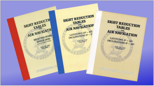
The PUB. NO. 249 consists of three volumes. The first volume covers the fixed stars and has to be reprinted every five years because the fixed stars are not so fixed. Volumes 2 and 3 cover the latitudes from 0° to 40° and 39° to 89° and they are always valid. In addition, there is PUB. NO. 229, which was compiled for maritime navigation. This table work is available in six volumes, each the size of a telephone book. The resolution is larger in these tables, which has necessitated more paper. Since a „Nautical Almanac“ was also always nessecary, is this all something for large ships rather than for use on the narrower sailing yachts.
It is noteworthy that the offer of the tables was suspended for a long time. Cruising yachtsmen and interested parties could only download them from the internet as PDFs. Volume 1, which becomes invalid after five years anyway because fixed stars are not fix, had long been nothing but wastepaper. But in the meantime all volumes are being printed again and published as books. The content of volume 1 has also been recreated and is now published again every five years. It almost seems as if the publishers have rediscovered the importance of astronavigation.

 

1.10 Artificial Celestial Bodies

When satellite navigation officially began operating in 1996, it was tantamount to a revolution. Positions could be found very quickly with the greatest of ease and accuracy. Soon every car had a road navigation system. Containers were given GPS trackers so that their location could be tracked around the world, and even toys like small drones were fitted with GPS tracking systems so that they could find their way back to the take-off site. The operator of the first satellite navigation system GPS (Global Position System) was the American military. It is not only used by ships and aircraft for navigation; it can also be used to guide combat drones and cruise missiles precisely to a target. Civilian use is only a side effect of all this.
Because of the military use by the Americans, Russia had to set up its own system GLONASS and the Europeans followed with Galileo. So, at present there are three independent systems that are also intended to make civilian use safer. In the meantime, we can look back on three decades of predominantly trouble-free peaceful operation. But how safe are these man-made systems really if their precision and function can be influenced by the operators at any time and could also be exposed to attacks by an enemy in the event of a conflict?

At the end of the 1990s, the Naval Academy in the USA suspended teaching astronomical navigation. No dangers were seen at the time. But a decade later, operational characteristics and weaknesses of the system were discovered that could make it unreliable or even unusable under certain conditions. For example, a satellite only has a certain lifespan after which its signal strength decreases. The danger that ageing satellites could not be replaced quickly enough for cost reasons became very real. The satellites‘ weak radio signals could also be disrupted, affected or even rendered useless by enemy action, cyber-attacks or a solar storm. Solar storms can affect a satellite’s controls, even causing it to crash. Another new threat is the increasing amount of space junk, which has the potential to destroy navigation satellites.
Because of these considerations, the concern spread that the growing dependence on fully electronic navigation could result in the complete loss of competence in astronomical navigation. The consequence was that in 2015, training in astronomical navigation was reintroduced at the Naval Academy in the USA. In contrast, the US Merchant Marine has never abandoned classical navigation with the sextant as an emergency system on its ships.
Although all these dangers are cited again and again, astronavigation as an emergency option is often suppressed or not taken seriously. Somehow it is also hard to imagine that aircraft carriers today would have to navigate with a sextant, as they did in World War II. But on a yacht, a simple power failure can put satellite navigation out of action, and without paper charts on board, even a location given by a smartphone is pretty useless.

1.11 Astronavigation Today

The dominant navigation system is satellite navigation. In addition, astronavigation continues to play a role as emergency navigation or as a hobby for all those who like to find their way with the help of nature and a sextant. This is particularly useful for sailors on long voyages. Another aspect is the preservation of maritime tradition, because sailing is also a traditional way of travelling on the water, and it is fitting if the skipper can still find his way with the sextant like the old sailors.
Many flag states have abolished the obligation to equip commercial vessels on long voyages with a sextant. The prerequisite for this, however, is redundancy in the form of a completely independent fully electronic secondary system. However, this cannot be guaranteed on countless yachts and smaller vessels. Sextant, nautical yearbook and knowledge of navigation are therefore still indispensable as back-up.
However, there are also other reactions from authorities. For example, in December 2019, New Zealand made it a legal requirement to carry a sextant and chronometer on seagoing boats over six meters in length. But if a skipper can’t do anything with it, it doesn’t help in terms of safety. For their own safety, cruising sailors in particular should therefore carry a navigation back-up on board.
In general, astronavigation is very unpopular. The main reason is certainly that those responsible in the countries had the honorable thought of wanting to maintain an emergency system alongside satellite navigation, but overlooked the fact that they had arrived in the computer age. Notwithstanding this, the use of tools from the last centuries was prescribed for the application of astronomical navigation.
If astronomical navigation is to be preserved as a fallback method, then it must be made usable. Usable sounds strange at first, because it was, after all, the navigation method used exclusively on all seagoing ships for longer as a whole century. But the competence to use it in the previous way is no longer available in today’s generation of seafarers. Nor can it be restored. For astronavigation to become usable again, it must be as simple as satellite navigation, apart from the additional use of a sextant, of course. Without question, this would benefit safety at sea.
How this is to be achieved has not yet been conveyed by the official side. Admittedly, there are numerous applications that help if navigation would have to be done with a sextant. You can find corresponding apps on the internet and in the Apple or Google stores. However, these are only calculation aids that enable a navigator to find position lines without using formulas. However, if you have little or no knowledge about the use of position lines, this will not help you. The invention of the position lines by Sumner and Hilaire was a stopgap at the time, which should actually be obsolete with the spread of the computer. The developers of satellite navigation knew better and got it right from the start.

What works for artificial celestial bodies must also be feasible for natural celestial bodies, i.e. without prior site guessing and without the construction of lines of position. Unfortunately, the algorithms required for this have never been discussed in the nautical literature of the last decades and are therefore hardly known, if at all. Common practice in the last two centuries has simply displaced them as „old“ procedures. However, they are a prerequisite for a new kind of astronomical navigation and therefore the topic in the following chapters.
First, however, an app is presented that works on the basis of a method developed by Carl Friedrich Gauss in 1808, 67 years or, in other words, almost three generations of navigators before Saint Hilaire. It is the first computer-based method of astronomical navigation that displays a location as a ship’s symbol on an electronic chart. No knowledge of mathematics or astronomy is required to use it.
This is made possible by limiting the navigation to the Sun. Only in this way can the app really be used by everyone. In principle, it would also be possible to use the moon, fixed stars and planets. However, this would require special knowledge of the entire starry sky, which only very few sailors have today. In the past, too, navigation was mostly based on the sun. Thus 90% of all celestial observations were solar observations. It would also be conceivable to use it in conjunction with a standard chart plotter. The extension of such a device, which is used on board almost all sailing yachts, would be done with an additional software module. This would allow any chart plotter to be converted to sextant navigation after an update. Programming a corresponding Astro module is not even complicated. However, it would be a task for the industry.