links → HOME, chapter 1, chapter 2, chapter 3, chapter 4, chapter 5 and 6, chapter 8
The position of the sun can only be used for navigation if the true solar time is also used. However, this deviates considerably from the time indicated by clocks known to us, such as ship’s chronometers, quartz clocks or atomic clocks, which are also called wheel clocks because of their uniform movement. The time indicated by wheel clocks runs absolutely evenly, but the earth does not move evenly as seen from the sun. It moves at different speeds in an elliptical orbit and its axis seems to wobble, which means that the length of the day between two solar noon peaks at the same place is different – slightly, but it adds up. The time indicated by evenly running clocks is therefore an average time compared with true solar time, because all irregularities even out again in the course of a year. True solar time is indicated by sundials, and it is well known that their time indications can advance or retard from those of a normal quartz wristwatch by a quarter of an hour in the course of a year.
Because the navigators only had the time indicated by a ship’s chronometer available for their work, they needed information about a time correction which, added to the chronometer time, provides the true solar time. This correction time or better compensation time is the equation of time. It is not an equation in the mathematical sense. Rather, it is the progression of a time function over a period of time, for example one year, which is necessary to balance the mean time indication of a wheel clock in order to obtain the true solar time from it. A practical form of application is a table with time data for each day at 12:00 UT1 of a year. The term equation of time is thus derived from its function of equalisation.
In our normal life, this is the other way round. There, the mean time determines our daily routine. Those who arrive ten minutes late cannot justify themselves by saying that they wanted to keep the appointment after the true solar time. It has been a very long time since people made their daily routine dependent on the course of the sun. Today, only a few sundials still bear witness to this. The existence of an equation of time was already suspected in antiquity. But it was only after Kepler’s laws became known that it became tangible and was calculated for the first time in 1672 by John Flamsteed (1646-1719). The secrets of this natural phenomenon, which is generally little known but is the most important basic requirement for navigation with the sun, will therefore be examined in more detail below.
7.1 Ellipticity of the Earth’s orbit
The equation of time is due to two independent causes. The first of these is the elliptical orbit of the Earth around the Sun. According to Kepler’s first law, the Earth orbits the Sun in an elliptical path, with the Sun at a focal point of this ellipse. The shape of the ellipse does not deviate significantly from a circle, as its numerical eccentricity is quite low at 0.0167. In a drawing true to scale, the actual elliptical orbit could not be distinguished optically from a circle at all. The representation in Figure 7.1 is therefore greatly exaggerated.

The Earth comes closest to the Sun in the northern winter. Then its disc also appears a little larger. In summer, it is at the greatest distance from the sun. The smallest and largest distances to the sun are the perihelion and aphelion, they form the ends of the main axis of the ellipse. However, they do not coincide exactly with the solstices. At the solstices, the Sun has its greatest northern and greatest southern altitude above the horizon, respectively. The perihelion is currently reached on 2 January, while the sun has its lowest position in the northern hemisphere already on 21 December, a few days before. The perihelion changes by about one day in 60 years.
At perihelion, the mass attraction between the Earth and the Sun is at its greatest. To prevent the Earth from crashing into the Sun as a result, it increases its orbital velocity and thus its centrifugal force to compensate for the increasing gravitational force. Kepler described this exactly in his second law:
„A driving ray drawn from the sun to the planet sweeps over equal areas in equal times.“
Figure 7.1 shows this schematically. The areas A1 and A2 are of equal size and are swept by a driving beam between the Earth and the Sun in a time interval t of equal size. Logically, the orbital velocity of the Earth is greatest when the longer distance is covered in the time t. The different orbital velocities have an effect on the distance covered.
The different orbital velocities have an effect on the equation of time. The Earth rotates very smoothly and a 360° rotation of the Earth around itself takes 23 hours, 56 minutes and 4.0905 seconds. This time is a sidereal day because the same starry sky always spreads out on a meridian after every one sidereal day. As the Earth rotates, it simultaneously moves a little further along its orbit around the Sun – and this has special effects.
Figure 7.2 shows the Earth in position 1, where the Sun culminates on a meridian just facing it. After several full Earth rotations of 360° each, the Earth is in position 2 and the same meridian that was still facing the centre of the Sun in position 1 is now pointing past the Sun towards the celestial sphere with the fixed stars. In order for the same meridian to always point exactly to the centre of the sun’s disc on a subsequent day, the earth must continue to rotate for about four minutes every day, which brings us to the 24 hours that a solar day lasts.

If only exactly four minutes are added to the sidereal day every day so that the sun culminates on the same meridian, this still does not explain a time difference between the wheel clock and solar time. This would be the case with an exactly circular Earth orbit. For this reason, we should also orientate ourselves on Figure 7.1. Near the Sun, the Earth moves faster on its orbit, which means that it advances a little further within a day’s time than when it is far from the Sun. As a result, it leaves the sun a little further behind on its path every day and therefore has to turn a little longer than four minutes every day. Towards summer in the northern hemisphere, the Earth moves away from the Sun again and its orbital speed decreases. It now covers somewhat shorter distances in each daily stage of its orbit. As a result, it no longer leaves the sun so far behind after each rotation. On the other hand, it now has to revolve less and its revolving times become shorter than four minutes.
The resulting change in the true length of the day between two days is a maximum of about ±8 seconds. Since the times add up, there is a maximum fluctuation of the true solar time of about ±7.5 minutes within a year in an approximately sinusoidal course.
7.2 Obliquity of the Ecliptic
A second cause of the difference between solar time and chronometer time is the obliquity of the ecliptic. The Earth’s axis is about 23.44° oblique to the plane of the ecliptic and thus also to the axis of the ecliptic. This position is almost invariable in relation to the fixed star sky. Seen from the Sun, however, the Earth’s axis appears to wobble. At the equinoxes it is at a maximum of +23.44° and -23.44° to the ecliptic axis as seen from the sun. At the solstices, it is still oblique to the ecliptic plane, but seen from the sun, both axes are congruent behind each other. On the other hand, the northern or southern hemisphere is inclined towards the sun and is illuminated more directly, which results in the seasons.

-
-
- Earth rotation: 0,25°/min or 15,00 NM/min at the equator
- Orbital velocity v: v = 0,986°/d oder 59,14 NM/d
- Declination δ: δ = 0° to 23,44° from 20. March to 21. June
-
At this point we would like to remind you of the zenith point of a celestial body. The zenith point of the sun is the place where an imaginary line between the centre of the sun and the centre of the earth breaks through the surface of the earth. It is the place where an observer sees the sun at its zenith.
After each revolution around itself, i.e. after a sidereal day, the Earth must continue to revolve for an average of about four minutes so that the Sun culminates on the same meridian of the previous day. This culmination meridian is located a little to the west of the zenith point after each rotation of the Earth around itself and before the start of the re-rotation. At the same time, the Earth has also progressed one day’s distance along its orbit during its rotation, as can be seen in Figure 7.4. This distance can be calculated. From the product of the orbital velocity of 0.986°/d and the rotational velocity of 60 NM/degree one gets
![\[s=\frac{0,986\,\text{Grad}}{d}\cdot\frac{60 \,\text{NM}}{\text{Grad}}=\frac{59,14\,\text{NM}}{d}\cdot\]](https://astro-navigation.com/wp-content/ql-cache/quicklatex.com-3d036c77ebccb4f953f6c836c00c903f_l3.png "Rendered by QuickLaTeX.com")
This distance is always in the plane of the ecliptic or perpendicular to the axis of the ecliptic. Two extremes can now be derived from this, which are shown on the left and right in Figure 7.4.
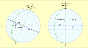
The process is as follows: at the equinoxes, on the left of the picture, the sun’s azimuth point hits the equator. As it progresses along its orbit, one of the Earth’s hemispheres tilts towards the Sun and the azimuth point moves north or south. As a result of the Earth’s rotation, it follows a spiral path on the Earth’s surface with increasingly close turns. In the picture, the beginning of the spiral path is indicated in yellow because the north pole in the example is leaning towards the sun. When the summer solstice is reached, a path is drawn along the tropic and parallel to the equator. Seen from the Sun, the Earth’s axis has become fully erect during this quarter of the year, as the image on its right shows.
Now we go back to the beginning of spring and thus to the left half of the picture. There, the culmination meridian from the previous day, shown in green, the equator section with length α and the daily leg of s = 59.14 NM, which here equates to a great circle with an zenith point track of 0.986°, form a right-angled spherical triangle, with the right angle existing between the meridian and the equator. In the triangle, the distance s is the hypotenuse and thus the longest side. The angle ε exists between the plane of the ecliptic and the equator. From this, the distance α can now be calculated. The earth still has to turn this distance on its axis so that the sun can culminate on the meridian drawn in green. The formula for calculating α is:
![\[\alpha=\arctan(\tan s\cdot\cos \epsilon)\]](https://astro-navigation.com/wp-content/ql-cache/quicklatex.com-d768a77b852cf264d20b6140605c396b_l3.png "Rendered by QuickLaTeX.com")
After substituting the numbers with s = 0.986° and ε = 23.44°, this calculates an angle α of 0.904°. With its rotation speed of 15°/h, the Earth needs exactly 3.618 minutes of after-rotation time until the meridian drawn in green reaches the zenith point or culmination point due to the Earth’s rotation. The difference to the average daily after-rotation time of 3.943 minutes is -19.51 seconds. This means that a solar day at the beginning of spring and also at the beginning of autumn is shorter than a mean solar day.
At the points of inflection, the northern or southern hemisphere is inclined towards the Sun and the Sun’s zenith point writes its track as a result of the Earth’s rotation on a tropic, with latitude  ≈ 23.44°, which at this point will have the magnitude of plus or minus ε. There the meridians are closer together and the zenith point track of 59.14 NM length drawn during a day’s leg on the orbit can sweep a larger angle or a larger meridian area. This angle is equal to the angle α on the equator, only there it has a greater length in nautical miles, which requires a longer sweep. The angle has the magnitude
![\[\alpha=\frac{s}{\cos\epsilon}\cdot\]](https://astro-navigation.com/wp-content/ql-cache/quicklatex.com-3c356f54d30f8f657d977be6892c14f7_l3.png "Rendered by QuickLaTeX.com")
After substituting the numbers, this results in a value of 1.075°, for which the earth has to turn for 4.299 minutes. This is then 21.32 s more than the mean rotation time and thus the solar day at the solstices is longer than the mean solar time by this time.
Starting from the beginning of spring, the daily seconds add up to about 9.85 minutes for about 46 days. This sum then decreases again to 0 in the further 46 days until the summer solstice. Because the ups and downs happen twice a year, there are two complete sinusoidal waves of time shift over the whole year.
7.3 Calculation Model
For a more accurate and comprehensive calculation, the Kepler model must be used. This is a two-mass model that only takes into account the masses of the Earth and the Sun and neglects the masses of the Moon and the major planets. However, deviations resulting from this are not significant. In a longitude calculation, they would cause errors of up to about  0.5′ and therefore do not play too great a role in practical navigation. Errors in the measurement of time and altitude cause larger deviations. Figure 7.5 shows the model suitable for calculation of a geocentric representation, of the Earth-Sun system as perceived from Earth.
Ultimately, it does not matter from which point of view the regularities are viewed. They are always the same. Only with regard to the view is it convenient to change the viewpoint and look at a geocentric model as in Figure 7.5 and a heliocentric model as in Figure 7.3. The model shows the celestial sphere with the rotating earth in the centre. The Sun S orbits the Earth once a year on its ecliptical path, which has the same inclination of ε to the celestial equator and also to the Earth’s equator, at a completely uniform speed.

Starting from the vernal equinox, which is one of the two intersections of the celestial equator and the ecliptic on the celestial sphere, the sun moves northwards and illuminates the northern hemisphere of the earth increasingly directly. It reaches its northernmost point at the summer solstice So and then moves southwards again on its path.
Exactly at the beginning of autumn, the second intersection of the equatorial plane and the plane of the ecliptic, the zenith point passes the equator and then continues to move southwards, with the sun illuminating the southern hemisphere more directly. Finally, the Sun passes the winter solstice Wi and reaches the vernal equinox again to complete the orbit.

On the celestial equator, a comparison sun Z should circle analogous to the hand of a large clock and with the same uniform orbital speed as the real sun. In addition, both suns pass the beginning of spring and the beginning of autumn at the same time. The respective meridian of the celestial sphere passing through the real sun meets the celestial equator at right angles, this intersection dividing the longitude αm into the sections α and g. The longitude of g is understood to be the equation of time.
However, there is a problem. Every time the sun reaches the vernal equinox again after a complete circulation, its zenith point hits a different meridian on the earth.
Thus, there is no number of 360° Earth rotations that fit into one circulation without remainder, especially since the Earth rotates slower and slower. Thus, every year begins on 1 January 00:00:00 UT on a different meridian.
This is exactly why you need a new table with the equation of time for every year or an almanac that is only valid for a certain year. So you have to ask when the earth started to turn, of course only in the calendrical sense. The answer is: on 1.1.4713 BC, almost 7000 years ago. That is how long calendars have been known in which the days are counted until today. However, there have been many calendar reforms in which the calendars were adapted to the solar year. In 45 BC, the Roman Emperor Gaius Julius Caesar reformed the Roman calendar that had been in use until then. In this new Julian calendar he created, a year had 365 days and every fourth year was a leap year with 366 days. This calendar lagged behind the astronomical reality based on the beginning of spring by one day every 128 years. Nevertheless, it is still used in some countries today.
In 1582, Pope Gregory reformed the calendar by simply skipping ten days, because the date of Easter was no longer determined by the beginning and full moon of spring. The leap year rule was also changed, so that although a leap day is added every four years, it is omitted at the turn of the century, unless the year is divisible by 400. Most countries have now adopted the Gregorian calendar. But the fact remains – there will never be a calendar in which the solar year and the calendar year coincide.
Stages were defined so that it would not always be necessary to calculate back to a day in the distant past. The last stage ended on 1 January 2000 at 12:00:00 UT1. For this reference date, the current values of the Earth’s orbital elements were stored as linear equations.
The equations are given in plate 7.1. They all have the form Y = A + B ⋅ T, i.e. they are linear equations of the first degree, where A is the constant of the respective parameter Y at the reference date and the product B ⋅ T describes the changes to be expected with the future days T.
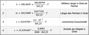
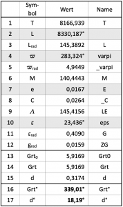
Table 7.1 contains all the important orbital elements defined at the reference date. In it mean:
-
- Mean longitude in degrees from perihelion is the point on the celestial equator reached by a point orbiting there when it is travelling uniformly like a clock hand at the mean orbital speed of the Sun from the reference date. Within 10 years, L then covers a distance of about 3600°.
- Longitude of perihelion in degrees is the point in the Earth’s orbit at which the Earth comes closest to the Sun in the northern winter. Longitude is measured in degrees from the vernal equinox.
- Numerical eccentricity is a parameter used to turn a circle into an ellipse, in our case a mathematical tool used to determine the elliptical orbit of the Earth around the Sun.
- Obliquity of the ecliptic in degrees is the angle that the plane of the ecliptic makes with respect to the horizontal plane. It is also the angle of the maximum possible declination of the Sun.
7.3.1 Determining Time as a Variable
For navigation, the sun’s positions – declination δ as deviation from the equator and hour angle GHA as longitude from a fixed prime meridian – are needed. It should be possible to calculate these from the orbital elements. It must be possible to calculate in advance the position of the sun or the coordinates of its zenith point on the earth’s surface, which is the same thing, for any second of any year. Only then will a navigator be able to calculate the coordinates of the sun’s zenith point with the help of a second-by-second determination of the sun’s altitude above the horizon. From the coordinates of two zenith points calculated at different times in relation to the Earth’s pole and his own position, which is still unknown, this can finally be determined.
The four orbital elements in Table 7.1 thus describe the position of the Sun on the ecliptic in relation to the Earth’s position, as a function of time T. Thus the first task is to calculate this time in days as a decimal number with an appropriate number of decimal places. The formula for this is:
(7.1) ![\[T=\mathbb{Z}\Bigr(\big(JJJJ-2000\big)\cdot 365,25\Bigr)+N-0,5+\frac{UT1}{24}-SJ\cdot\]](https://astro-navigation.com/wp-content/ql-cache/quicklatex.com-fda664b8bdccaa3833d464065b1a1564_l3.png "Rendered by QuickLaTeX.com")
In this, the leap year definition
(7.2) ![\[SJ=\text{wenn}\;4|(JJJJ -2000)\;\text{dann}\;1\;\text{sonst}\;0\cdot\]](https://astro-navigation.com/wp-content/ql-cache/quicklatex.com-e851a2a115f8511dcfb9075b6972f067_l3.png "Rendered by QuickLaTeX.com")
applies until 2099. ℤ means the integer part of the value that is in the following parenthesis. Thus, the year 2022 in the large bracket yields the value 8035.5. Then ℤ = 8035 because the decimal part of 0.5 is simply omitted. The 2000 to be subtracted is the year of the reference date.
N denotes the days that have passed in the year under consideration, including the current day. Thus N on a 12 February is 43 days. The -0.5 days are necessary because the sun does not culminate at 0 o’clock on the prime meridian, but at noon. This is an arbitrary determination based on the tradition that 12 o’clock is noon and the sun is at its highest at noon.
The following fraction UT1/24 determines the fractional part of the day with the decimal number of UT1. SJ refers to the leap year rule described in equation 7.2, which applies in this simplified form until 2099. According to this rule, there is always a leap year if the year number is divisible by four without a remainder. This equation is read as:
If 4 is the divisor of (YYYY – 2000), then 1, if not, then 0.
Thus, every fourth year is a leap year in which one day must be subtracted. Subtraction is called for because when multiplying by 365.25, the decimal value of 0.25 produces an additional day every four years. The year 2100 is not a leap year, although it is divisible by 4. However, it is also divisible by 100 and therefore fails as a leap year. The rule with equation 7.2 therefore only applies until the year 2099.
To measure time, people use mechanical clocks that run very evenly. The course of time indicated by these clocks can be compared with the course of the imagin reference sun Z in Figure 7.5, whose zenith point never leaves the equator, but always covers the same difference in longitude per unit of time. This is not the case with the real sun, because for it it is always a different difference in longitude per unit of time.
If we assume its speed on the orbit to be constant, then its zenith point crosses more meridians in the same time when it faces the northern or southern hemisphere than when it faces the equator, where the meridians are furthest apart. The longitude on which the zenith point of the true sun is currently located differs from the longitude on which the zenith point of the comparison sun is located by the amount g shown in Figure 7.5. This difference in longitude is the equation of time because 1° difference in longitude is the same as four minutes of solar transit time. So when it comes to determining the zenith point length of the true sun with the time indication of a wheel clock, its time indication is an average time and the true solar time is only obtained by adding the equation of time.
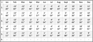
Earlier navigators had the equation of time for each year available in the form of a table, as shown here as an excerpt in table 7.2. A navigator determined the hour angle of the sun according to the time indicated by a chronometer, which he had to correct with the equation of time. If the difference in the amount of correction from one day to the next was too great, then it even had to be converted to the hour of observation. Later, the effort of this conversion was remedied by issuing tables in which the hourly angle was given for each day in the hourly grid. These were then the Nautical Almanacs.
7.3.2 Calculation of the Equation of Time
According to Figure 7.5, the equation of time is simply the resolution of the relation
(7.3) ![\[g=\alpha_m-\alpha\cdot\]](https://astro-navigation.com/wp-content/ql-cache/quicklatex.com-6e89e4fe7143f38aefb607df1d9fd4ae_l3.png "Rendered by QuickLaTeX.com")
By αm we mean the principal angle of longitude L. For example, at the beginning of July 2021 the Earth has already performed its orbit around the Sun about 21.5 times, each 360°, and that would be just under 21.5 ⋅ 360° = 7740° plus the 280° from the vernal equinox to perihelion. In total, that would be 8020°. The exact number is provided by the orbital element L. The main angle is obtained by taking full 360° revolutions out of the number. The following formula then applies:
(7.4) ![\[\alpha_m=L-\mathbb{Z}\Bigg(\frac{L}{360^\circ}\Bigg)\cdot 360^\circ\cdot\]](https://astro-navigation.com/wp-content/ql-cache/quicklatex.com-0f4e186dbd19e14a39696d5acece1720_l3.png "Rendered by QuickLaTeX.com")
With the calculation of α, things get more complicated. As Figure 7.5 shows, Λ, α and δ, all being great circle segments, form a right-angled spherical triangle with the right angle between α and the meridian passing through the Sun. For this triangle, the calculation formula is quickly found in a formula book with tan α = tan Λ ・ cos ε.
Taking into account the full circularity, however, it is more convenient to use the transformation formula
(7.5) 
to work. One would otherwise be confronted with too many overflows. The subscript Λ in the arc function calls the angle closest to Λ. This formula is then to be used as follows:
(7.6) ![\[\alpha=\arctan_\Lambda(x)=\arctan(x)+\pi\cdot \mathbb{Z}\Bigg(\frac{\Lambda-\arctan(x)}{\pi}\Bigg)\cdot\]](https://astro-navigation.com/wp-content/ql-cache/quicklatex.com-f55c88f7094586bb71f68a4d95f4f61e_l3.png "Rendered by QuickLaTeX.com")
In this is  . To be able to solve the equation, Λ is needed and for this:
(7.7) 
With C, the so-called midpoint equation comes into play here, which is used to calculate an elliptical orbit by elliptical deformation of a circular orbit. According to Kepler, it depends on the eccentricity e of the respective orbital ellipse and is the difference between the mean anomaly M and the true anomaly V. However, we will not go into this further here. The mean anomaly is the difference between the mean length and the length of the perihelion. The following applies:
(7.8) 
The additional full circle angle of 360° in this equation does not matter, since only the sine of M is used in the following. It is then completely the same how often 360° are added to it. The formula M = L –  would also give the same result, which just could not be reproduced so easily graphically.
Since the Kepler equation can only be solved iteratively and the eccentricity of the Earth’s orbit is quite small with e = 0.0168, a series development makes more sense here. In the literature, one finds for this:
![\[C=\frac{180}{\pi}\Bigg((2e-\frac{e^3}{4})\cdot\sin M+\frac{5}{4}e^2\cdot\sin (2M)+\frac{13}{12}e^3\cdot\sin (3M)+\]](https://astro-navigation.com/wp-content/ql-cache/quicklatex.com-ad475094ffce712a3a61dc223ca2d788_l3.png "Rendered by QuickLaTeX.com")
(7.9) ![\[+\frac{103}{96}e^4\cdot\sin 4M+\frac{1097}{960}e^5\cdot\sin (5M)\Bigg)\cdot\]](https://astro-navigation.com/wp-content/ql-cache/quicklatex.com-679e032dac5acd501b1b11f011be5e0e_l3.png "Rendered by QuickLaTeX.com")
The third line of this equation or the last two sums in the parenthesis can also be omitted. They no longer make a significant contribution to the result. With the result, Λ can now be calculated according to equation 7.7 and, after calculating equation 7.5 using the solution aid in equation 7.6, yields the length α. Equation 7.3 can then be used to give the equation of time in degrees. Multiplying by four also gives the result in minutes of time, as given, for example, in plate 7.2.
As already described, the equation of time depends on the eccentricity and on the ecliptic obliquity, i.e. on two components. The contribution from the orbital eccentricity is calculated by placing the ecliptic axis and the Earth’s axis parallel. The following applies:
(7.10) ![\[g_{\epsilon=0}=\alpha_m-\Lambda\cdot\]](https://astro-navigation.com/wp-content/ql-cache/quicklatex.com-aa7cbef29e57a921d6b15660918b97ee_l3.png "Rendered by QuickLaTeX.com")
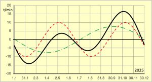
This part is sinusoidal with a period in one year. It is the green dash-dot curve in Figure 7.7 and is also obtained from Eq. 7.8 by rearranging -C = αm – Δ as -C .
The second component is the contribution due to the obliquity of the ecliptic and is obtained as:
(7.11) ![\[g_\epsilon=\Lambda-\alpha\cdot\]](https://astro-navigation.com/wp-content/ql-cache/quicklatex.com-0eda2fb9d5f0b430bf43a5fddcd9e874_l3.png "Rendered by QuickLaTeX.com")
The application of the arc tangent with position parameter according to equation 7.6 does not prevent numerical values from occurring here that exceed expectations. However, values exceeding 0.07 – corresponding to 4° – are not expected under any circumstances. Should numbers be calculated that exceed this maximum, then  must be subtracted from the result of the equation. The course is, as already mentioned above, also sinusoidal, but with two periods in one year. This is shown in Figure 7.7 as a red dashed curve.
The equation of time is the sum of the components described with equations 7.10 and 7.11 and thus
(7.12) ![\[g=g_{\epsilon=0}+g_\epsilon=\alpha_m-\alpha\cdot\]](https://astro-navigation.com/wp-content/ql-cache/quicklatex.com-2278f861ef5286136a05e76748b5485c_l3.png "Rendered by QuickLaTeX.com")
The result is, as expected, Eq. 7.3 and drawn as a solid black curve in Figure 7.7.
If the equation of time components are not to be calculated individually, but the equation of time is to be calculated completely and directly, which is sufficient for practical use, then the transformation described below will help. By replacing α in Eq. 7.12 or 7.3 with Eq. 7.5, the equation of time can also be given in more detail:
![\[g=\alpha_m-\arctan_\Lambda(\tan\Lambda\cdot\cos\epsilon)\cdot\]](https://astro-navigation.com/wp-content/ql-cache/quicklatex.com-8a50a65e4f2765d8a9f47c042ceb2f58_l3.png "Rendered by QuickLaTeX.com")
A tangent addition theorem is:
![\[\tan(x-y)=\frac{\tan x-\tan y}{1+\tan x\cdot\tan y}\]](https://astro-navigation.com/wp-content/ql-cache/quicklatex.com-e5dd0564bce23a24eda83e8d24936c55_l3.png "Rendered by QuickLaTeX.com")
The tangent inverse function yields for this:
![\[x-y=\arctan\frac{\tan x-\tan y}{1+\tan x\cdot\tan y}\]](https://astro-navigation.com/wp-content/ql-cache/quicklatex.com-d8b48d53967a13cb2b5fabc92b5ab1fd_l3.png "Rendered by QuickLaTeX.com")
With  and
and
 it follows:
(7.13) ![\[g=\arctan\frac{\tan \alpha_m-\tan \Lambda\cdot\cos \epsilon}{1+\tan \alpha_m\cdot\tan \Lambda\cdot\cos \epsilon}\cdot\]](https://astro-navigation.com/wp-content/ql-cache/quicklatex.com-81f68e41b358cf216ea91d0b20745f76_l3.png "Rendered by QuickLaTeX.com")
All equations given so far deliver angular data and these even almost always in radians, as radians. The corresponding time data are obtained from this after multiplication by 4 min/degree.
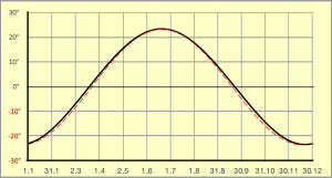
Figure 7.7 shows the course of the equation of the year 2025. The two components are shown in colour. The green interrupted line is due to the ellipticity of the Earth’s orbit according to equation 7.10 and the red interrupted line is the result of the obliquity of the ecliptic according to equation 7.11. By adding the function values, one obtains the combined equation of time, which is shown as a black curve according to equations 7.12 and 7.13. The four zero crossings of this curve are shown in Figure 7.7.
It can be seen from the four zero crossings of this curve that the true solar time only agrees with the time of a wheel clock on four days a year and can otherwise be up to a quarter of an hour ahead or behind. Knowledge of the equation of time is indispensable for determining a position with the sun at sea.
7.4 The Ephemeris of the Sun
This refers to the position of the Sun on the celestial sphere or its zenith point on Earth. This position is described by a longitude component, the Greenwich angle, and a latitude component, the declination.
The division of the Earth’s grid of degrees into 180 positive east degrees and 180 negative west degrees was not optimal in terms of navigation because it did not match the course of the Sun. The hour angle would first count down from 180° E to zero degrees at the zero meridian and then further into the negative to 180° or -180° W. An hour angle was needed that, starting from the zero meridian and counting upwards from 0° to 360° with the course of the sun to the west, would go once around the earth. Parallel to this, a clock was to turn its 24 hours.
The prime meridian was established in 1884 at the Meridian Conference in Chicago as the one that passes through the Greenwich Observatory. The hour angle progressing westwards from this was called – as already mentioned – Greenwich Hour Angle, or GHA for short.
Unfortunately, the time could not be adjusted so that it was always 00:00 when the sun started at the prime meridian. Its start had to begin with a clearly definable event in its course, and that is only the culmination. However, the sun culminates at 12:00 and this is noon according to the bourgeois conception of time. To do justice to everything, the start of the sun at the prime meridian was set at midday. Due to the equation of time, however, the sun only passes the prime meridian at exactly 12:00 noon in the year only four times.
Navigation with the sun only works with true solar time, which is obtained by adding chronometer time and the equation of time. The further arithmetic involved only the basic arithmetic operations, but could also become tedious. For example, Table 7.2 gives a deviation of 18′ and 26“for the 4th of Nov. That is then about 0.75 minutes change per hour, which is already quite significant. This conversion of the equation of time to the hour of the day was overcome with the creation of the solar almanac.
7.4.1 Greenwich Angle GHA
To obtain the Greenwich angle for the time of a solar observation, 12 hours have to be subtracted from the sum of chronometer time and equation of time and the result multiplied by the zenith point velocity of 15°/h. The Greenwich angle is then calculated from the equation of time.
Another possibility is to consider primarily not the times, but these equal as hour angles in degrees, in which case four minutes equal one degree. The ordinate of the equation of time in Figure 7.7 would then not be scaled in \pm16 min, but in \pm 4°. The same is then done with the chronometer time, so from 12:00 onwards every 4 min equals 1 degree. This gives each full hour after 12:00 a formal hour angle increase of 15°.
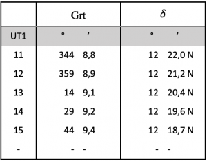
If now – in a table – the equation of time converted into degrees is added to each of these evenly running full hour angles, then a Sun Almanac results. The advantage of this is less calculation work, but more searching in a new set of tables, which must have an extra table for each day of the year. Table 7.3 shows its basic structure with figures from 20 August 2022.
The first column contains the universal time UT1. This is adapted to the Earth’s rotation and is the reference time for the completely uniform UTC or atomic clock time, which is equated with the chronometer time on board. Since the earth rotates more and more slowly, the UTC must be adjusted to UT1 ever after several years. The second column then shows the GHA in degrees and minutes. In this way, you can get the GHA without having to convert the chronometer time beforehand. For the minutes and seconds of an observation hour, interpolation is necessary, which can be done with the help of specials tables at the end of the Almanac.
In this way, the Greenwich angle starts at the prime meridian and counts 360° around the globe. Since the day starts at 180° E, but the prime meridian is 180° further west, this offset must be taken into account with 12h. The GHA is calculated with the following formula:
![\[GHA=g+15\cdot\big(t+12^h\big),\]](https://astro-navigation.com/wp-content/ql-cache/quicklatex.com-36c18820a33b1d942881350c334be037_l3.png "Rendered by QuickLaTeX.com")
(7.14) ![\[GHA=g+15\cdot\big(t+12^h\big)\cdot\]](https://astro-navigation.com/wp-content/ql-cache/quicklatex.com-104c7b5d3b204651ab47e22256399fb0_l3.png "Rendered by QuickLaTeX.com")
In this, t is the time UT1 of the day in the 24-hour run for which the GHA is to be calculated. The time 12h is the time taken by the sun to travel from 180° E to the prime meridian.
The expression below it says that the contents of the parentheses must not be greater than 24h. For afternoon times, 24 hours must therefore always be subtracted. 15 means the angular velocity of the sun of 15°/h and g is the equation of time in degrees according to equation 7.13.
7.4.2 Deklination δ
The first declination tables already existed in the Middle Ages. They were imagined as a sine wave that had a zero crossing at the equinoxes and reached its respective maximum values of 23.44° at the solstices. That was about right, as Figure 7.8 shows. In fact, however, it is an approximation because this assumption ignores the effect of the equation of time. The declination can easily be calculated exactly. In Figure 7.5 it is easy to see that the triangle with sides δ, Λ and α is a right triangle. The right angle exists between the sides α and δ and the side δ can therefore be easily calculated with a simple formula from the formula book. By substituting the appropriate quantities one obtains:
(7.15) ![\[\delta=\arcsin(\sin\epsilon\cdot\sin\Lambda)\cdot\]](https://astro-navigation.com/wp-content/ql-cache/quicklatex.com-d5c013ebeb4df7da18418ed0e1e3c613_l3.png "Rendered by QuickLaTeX.com")
The length Λ is given by equation 7.7. Multiplication by the quotient 180°/\pi gives the angle in degrees. A small section of the declinations on 20 August 2022 is shown in Plate 7.3, also in the right-hand column.
7.4.3 The Nautical Almanac
A nautical almanac, however, is much more extensive. It has a so-called day page for each day of the year. On this page, the positions of the stars are given as the Greenwich hour angle GHA, the declination δ in the hour grid for the sun and the moon, and the four planets suitable for navigation. For navigation with fixed stars, the ♈︎GHA is required, which is the GHA of the vernal equinox. If this is added to the star angle of a fixed star given as β, then the GHA of the fixed star is obtained.
However, the positions of a fixed star are not as fixed as once thought. Thus, the star angle of some fixed stars must also be specified anew from year to year.
But a nautical yearbook contains even more. Because the hourly angles are only given in the hourly grid, the minutes and seconds of an observation time must be interpolated. For this purpose, so-called switching tables are provided at the end of the book so that no calculations have to be made here either. The tables for a sextant feed are also important. In addition, the equation of time table of the year is always given, furthermore the error corrections for the north star latitude and much more.
This effort with the switchboards is necessary to avoid errors as much as possible. You didn’t have to calculate so much, but you had to leaf through the pages all the more. This had its advantages especially in the case that a skipper, plagued by seasickness, was no longer able to do even the simplest mental arithmetic.
The first German edition of a nautical yearbook was published in 1852 by the German Hydrographic Institute in Hamburg. The name of this office later changed to the Federal Maritime and Hydrographic Agency (BSH). The last edition was published in 2020, thus ending an old tradition.
Today, large-scale shipping only uses fully electronic satellite navigation. Documents for astronomical navigation and also a sextant are no longer mandatory equipment in large-scale shipping, provided that two completely independent fully electronic satellite navigation systems are operated on board.
In the Basic version, the Sun Navigation app uses a calculation routine with which the solar ephemerides are calculated within milliseconds from the orbital elements in plate 7.1 and the entered observation time, consisting of date and time of day. The Pro version has a database in which the solar ephemerides are kept up to and including 31 December 2040. There is no need to calculate or scroll here.
7.4.4 Ephemeris of the Sun calculated with MS Excel
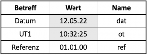
Everyone probably has the MS Office programme Excel on their home PC and with it it should be possible to calculate GHA and δ for any time in this century. That means: We now want to calculate the position where the sun is at its zenith at a given time and date. We also take an example right away, 12 May 2022 at 10:32:25 UT1 (similar to UTC).
We only need three small tables for this. The first table, table 7.4, has three rows. The first two rows are for entering the date and time for which we want to calculate the ephemeris. In the third row we write the reference date, 1 January 2000. The values of the data cells are assigned the names dat, ot and ref, which we then also write in the third column behind them.
In the second table, Table 7.5, we store the orbital elements of the Earth from Table 7.1.
These are the values A on the key date and the coefficients B, which cause a summation for a later time T. Here, too, it is most practical to first assign the names in the third column. We choose the names _A1 to _A4 and _B1 to _B4. The underscore before the letters A and B prevents confusion with the worksheet cells A1 to B4. The values for _A1 to _A4 are the constants indicated in Table 7.1 and can be copied directly from there.
The coefficients _B1 to _B4 are the fractions given in Table 7.1, which must first be converted into decimal fractions before being used. For all those who have little experience with Excel, this is shown for the coefficient B3, which has been given the name _B3. Click on the cell to the left of the name _B3 and enter the fraction in front of the time T in Table 7.1: =4.2E-7/365.25.
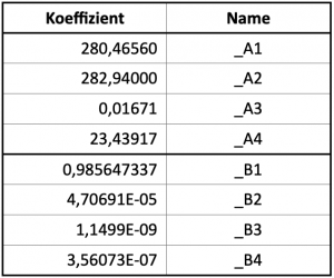
Excel calculates 1.1499E-09 from this, i.e. a decimal number with the power of ten 10-9. This is now also done for all other B values.
Now we just have to tell Excel the names we have given it. To do this, we click on the cell with the number for which the name is to apply. For example, in panel 7.4 we click on the date 12.05.22, because the name dat is to be given to Excel for this date. Then click on the function Formulas in the upper green function line and select the drop-down menu Define Names. Then select Define Names again. A window opens in which the name dat is entered in the line „Enter a name for the data area:“ and confirmed with OK.
The same is then repeated for all other cells. Finally, all cells with the values or coefficients should be selected one after the other. If everything has been done correctly, the name given to the selected number always appears in the input bar at the top left. If the cell with the number 0.0167 is selected, the name _A3 appears in the top left corner.
Next, the calculation table is set up, which can be seen here as panel 7.6. The table has 17 rows and three columns. Just as with the previous tables, Excel must be told the names defined in the name column so that the formulas in the value column can access them. All the formulas to be entered in the values column of Table 7.6 are given in the notation required for Excel in Table 7.7.
In line 1, the time T is first calculated. Excel has a special formula for this that is much simpler than the general equations given in equations 7.1 and 7.2. In the application it reads =TAGE(dat;ref)+ot-0.5.
From this Excel can now calculate all four orbital elements for the date and time of day as given in Table 7.4. The general formula Y = A + B ⋅ T of the orbital elements in Table 7.1 is applied to the respective special parameters and the time T in the value column in rows 2, 4, 7 and 10 (grey background). Except for the value of the numerical eccentricity e in line 7, the other angles calculated in degrees are converted to radians in the cell below. To convert, simply multiply the degrees from the cells above by /180.
In Excel there is also the formula Wrad = radians(W°). Note that the constant is always specified as PI() in Excel. The brackets behind it have no further meaning.
The difference between the mean length αm and the length of the perihelion provides the mean anomaly M with equation 7.8 in line 6. With its value and the numerical eccentricity e from line 7, Excel now calculates the midpoint equation C with equation 7.9 in line 8. In line 14, this is used to calculate the ecliptic longitude Λ as the sum of C and αm or L.
Finally, everything is then together to calculate the equation of time g with the equation 7.13 standing in line 12. It then follows with equation 7.14 entered in line 13 to calculate and display a GHA0. This is a value that has arisen in a first calculation step and could have a negative overflow. If GHA0 is less than zero, then 2 must be added. Line 14, which is used for correction in this case, then contains the correct GHA in radians. By multiplying with 180/, or in Excel also with the formula degrees of GHArad, the Greenwich angle is also given in line 16 in degrees.
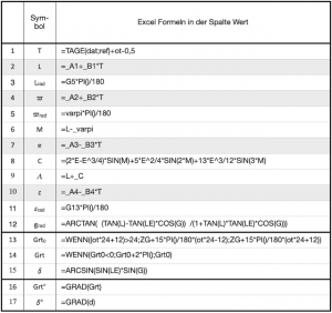
The declination δ, here denoted by the name d, is calculated with equation 7.15, which in Excel notation is in line 15. The degree measure of the declination is obtained in the same way after multiplication by 180/ or as a degree of GHArad in line 17.
In Excel there is another special feature for time calculations. For example, in the formula for GHA0, the time of day ot is multiplied by 24, which may seem surprising at first. The reason for this is that Excel calculates with 24 h = 1 and thus 1 hour = 1/24 and 12:00 = 0.5. The factor 15*PI()/180 also used there corresponds to (15°/h ⋅ /180) and is the angular velocity of the sun. This makes the formula in line 13 look a bit confusing.
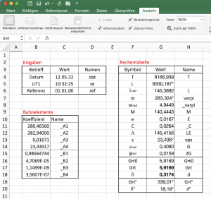
Figure 7.9 shows how the three tables can be arranged in an Excel worksheet. They take up surprisingly little space there.
The calculation table shows all the results of the numerical example entered in plate 7.4. The ephemerides GHA and δ are searched for the
12 May 2022 at 10:32:25 UT1.
The result is given in the last two lines of the arithmetic table. It is GHA = 339.01° and δ = 18.19°. A conversion from decimal degrees to degrees and minutes is done by subtracting the number of degrees before the decimal point and multiplying the difference by 60, which gives the minutes. However, this requires more than just two digits after the decimal point. After that we get
GHA = 339° 0.77′; δ = 018° 11.24′ N.
This simple calculation method according to Kepler only takes into account the masses of the Sun and the Earth. No account is taken of the influences of the Moon and the major planets. Therefore, ephemerides calculated with this method deviate somewhat from the actual position. However, the resulting location errors are not significant. Errors due to not careful altitude and time data usually have greater effects.